|
|
|
|
April 7 2006 GIPS test report
|
|
|
|
|
 | release candidate RC_20060131
|
|
|
|
|
|
 | location of test artifacts/ output data:
|
|
|
|
|
|
| Input data files:
1320_01_01_ifg.nc -- Earth data cube
1320_hbb_1_1_ifg.cdf -- hot blackbody data cube
1320_wbb_1_1_ifg.cdf -- warm blackbody data cube
1320_sbb_1_1_ifg.cdf -- space blackbody data cube
|
|
|
|
|
|
| Purpose: This test demonstrates the ability of the GIPS data processing pipeline to process simulated data cubes, and compares the output to the TOA radiances used to generate the input interferogram.
SimCal3 test script - generates output spectra:
#!/bin/sh
time ./simcal3 H /home/rayg/Workspace/mpi_earth_sequence_1/1320_hbb_1_1_ifg.cdf W /home/rayg/Workspace/mpi_earth_sequence_1/1320_wbb_1_1_ifg.cdf S /home/rayg/Workspace/mpi_earth_sequence_1/1320_sbb_1_1_ifg.cdf E /home/rayg/Workspace/mpi_earth_sequence_1/1320_01_01_ifg.cdf
|
|
|
|
|
|
| location of output and test artifacts:
|
|
|
|
|
|
| flenser.ssec.wisc.edu: /home2/projects/data/gips_test/20060406/
|
|
|
|
|
|
| listing of output files with explanations:
|
|
|
|
|
|
| 1320_01_01_apodized.nc - apodized GIPS output - main test artifact.
1320_01_01_ifg_unresampled.nc - GIPS intermediate product (data after radiometric calibration, before resampling)
1320_01_01_ifg.nc - unapodized GIPS ouptut
fd8_20030624_1320_01_01_rad.cdf - TOA radiance file for comparison
|
|
|
|
|
|
| Preliminary look at data, using MATLAB:
|
|
|
|
|
|
| >> fa = netcdf('1320_01_01_apodized.nc'); fr = netcdf('fd8_20030624_1320_01_01_rad.cdf'); fs = netcdf('1320_01_01_ifg.nc');
|
|
|
|
|
|
| >> al = fa{'signalReal_lw'}(:,:,:); ar = fr{'radiance'}(:,:,1:1024); as = fs{'signalReal_lw'}(:,:,:);
|
|
|
|
|
|
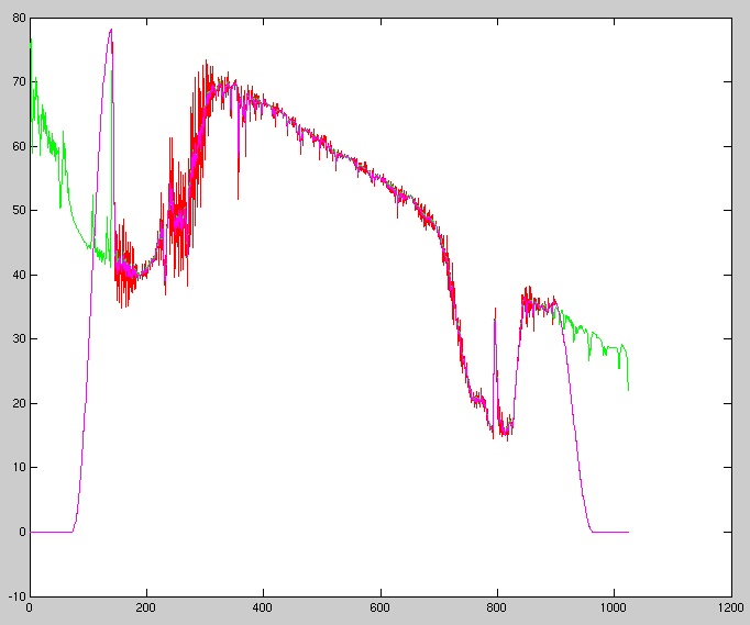
| Plot of pixel (50,50)
green: reference TOA radiance
red: unapodized GIPS output
magenta: apodized GIPS output
>> al50 = squeeze(al(50,50,:)); ar50 = squeeze(ar(50,50,:)); as50 = squeeze(as(50,50,:));
>> plot(as50,'r'); hold; plot(ar50, 'g'); plot(al50,'m');
|
|
|
|
|
|
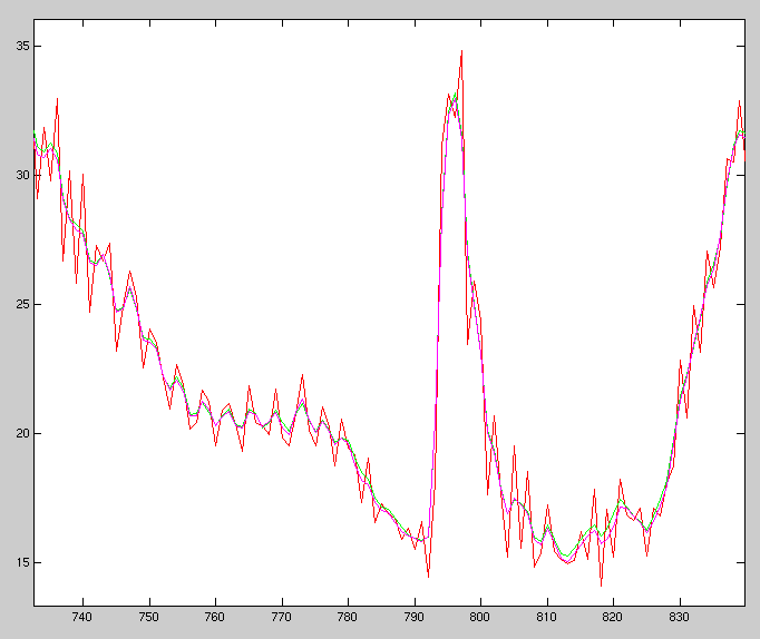
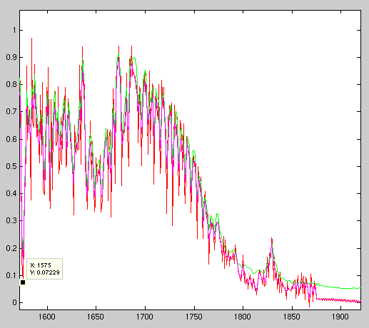
| Zoom of above graph, in window region:
|
|
|
|
|
|
| for whole-cube analysis, limit data to points 146 - 895 (within rolloff region)
|
|
|
|
|
|
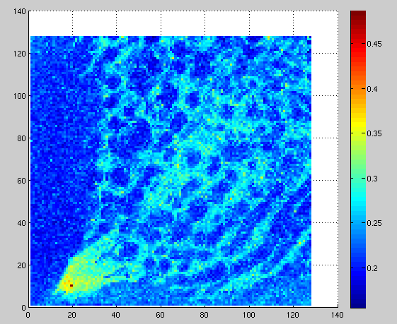
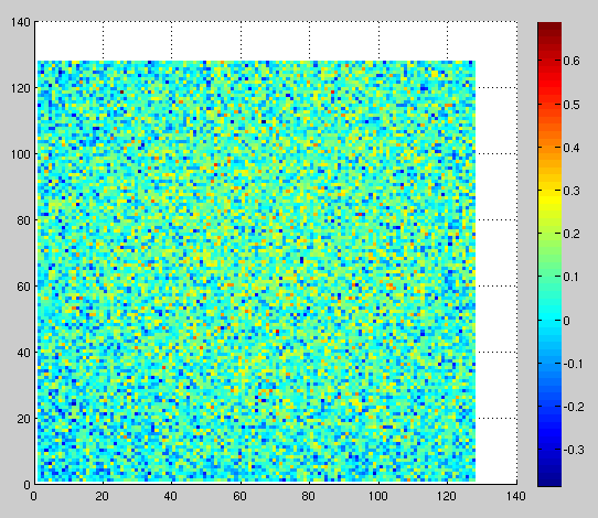
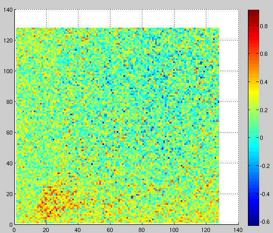
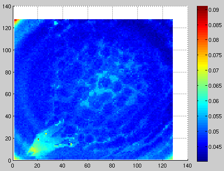
| RMS difference between apodized GIPS output and reference TOA radiances across entire cube
>> darl = ar(:,:,146:895) - al(:,:,146:895); sdarl = darl.^2; msdarl = mean(sdarl,3); rmsdarl = msdarl.^(.5);
>> surf(rmsdarl); view(2); shading flat; colorbar
|
|
|
|
|
|
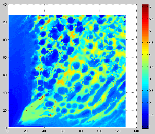
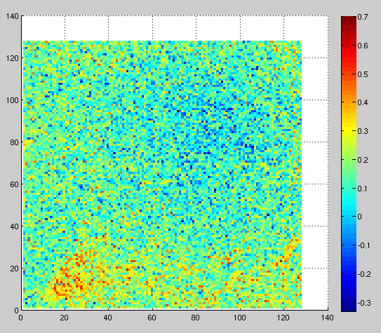
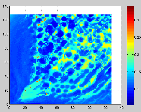
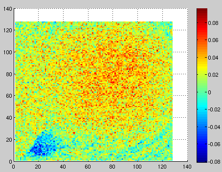
| To see the difference that apodization makes, compare with:
|
|
|
|
|
|
| RMS difference between unapodized GIPS output and reference TOA radiances across entire cube
>> rmsdsrl = (mean((ar(:,:,146:895) - as(:,:,146:895)).^2,3)).^(0.5);
>> surf(rmsdsrl); view(2); shading flat; colorbar
|
|
|
|
|
|
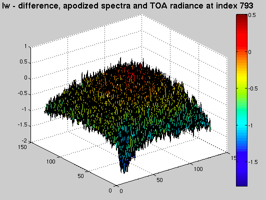
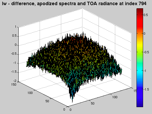
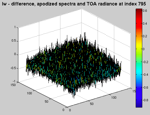
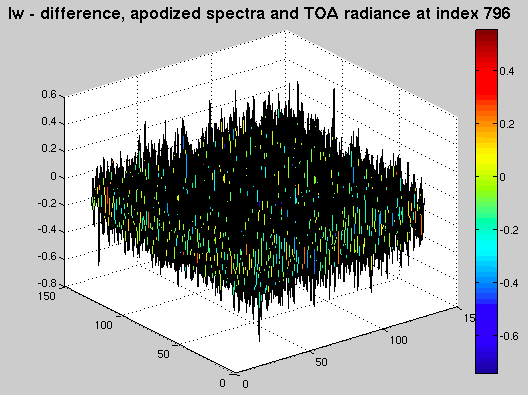
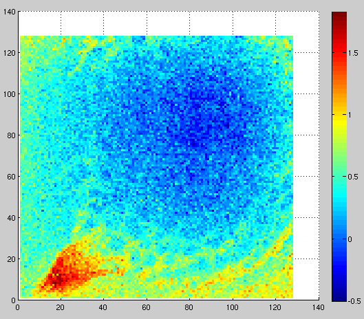
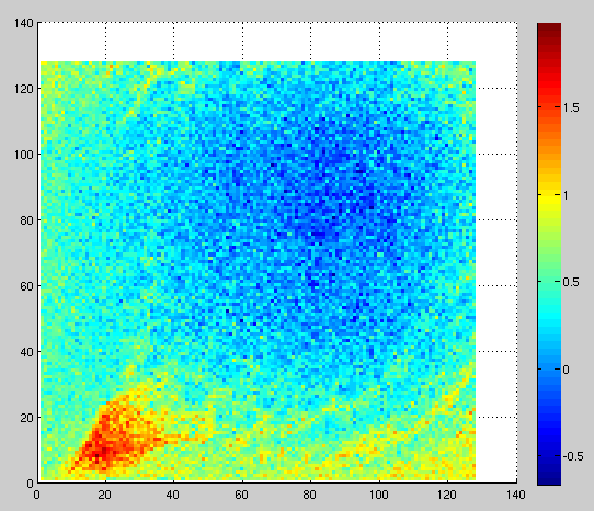
| To see the limits of resampling effectiveness (possibly having to do with a small error in calculating Theta between the simulator and GIPS), consider the following series of consecutive single wavenumber cross sections through the cube, centered around the prominent spike in the middle of the ozone region:
|
|
|
|
|
|
| >> surf(squeeze(darl(:,:,792-146))); view(2); shading flat; colorbar
|
|
|
|
 |
|
|
| >> surf(squeeze(darl(:,:,793-146))); view(2); shading flat; colorbar
|
|
|
|
|
|
|
| >> surf(squeeze(darl(:,:,794-146))); view(2); shading flat; colorbar
|
|
|
|
|
|
|
| >> surf(squeeze(darl(:,:,795-146))); view(2); shading flat; colorbar
|
|
|
|
|
|
|
| >> surf(squeeze(darl(:,:,796-146))); view(2); shading flat; colorbar
|
|
|
|
|
|
| Short-medium wave band brief analysis:
|
|
|
|
|
|
| >> am = fa{'signalReal_mw'}(:,:,:); rm = fr{'radiance'}(:,:,1025:3072); sm = fs{'signalReal_mw'}(:,:,:);
>> am50 = squeeze(am(50,50,:)); rm50 = squeeze(rm(50,50,:)); sm50 = squeeze(sm(50,50,:));
|
|
|
|
|
|
| Single pixel (50,50) plot. green: TOA Radiance, red: unapodized GIPS output, magenta: apodized GIPS output.
>> plot(sm50,'r'); hold; plot(rm50, 'g'); plot(am50,'m');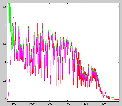
|
|
|
|
|
|
| Zoom in on tail end, which appears to peel off from the reference TOA radiances:
|
|
|
|
|
|
| RMS of difference between TOA rads and unapodized GIPS output, SM band:
>> rmsdsrm = (mean((rm(:,:,797:1873) - sm(:,:,797:1873)).^2,3)).^(0.5);
>> surf(rmsdsrm); view(2); shading flat; colorbar
|
|
|
|
|
|
| RMS of difference between TOA rads and apodized GIPS output, SM band:
>> rmsdarm = (mean((rm(:,:,797:1873) - am(:,:,797:1873)).^2,3)).^(0.5);
>> surf(rmsdarm); view(2); shading flat; colorbar
|
|
|
|
|
|
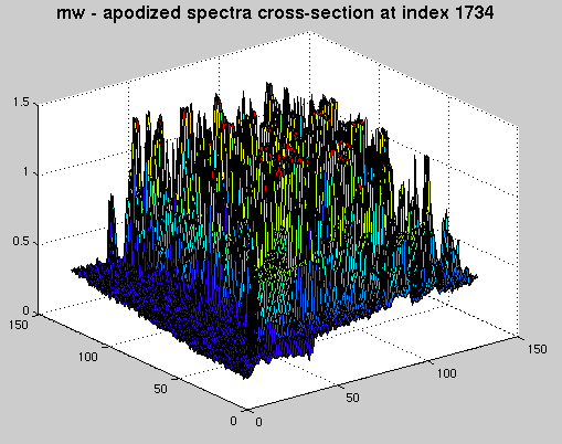
| Sample cross section through cube at a single channel:
>> surf(squeeze(darm(:,:,1734))); view(2); shading flat; colorbar
|
|
|
|
|
|
| Graphical results from running automated test report tool on same data:
|
|
|
|
|
|
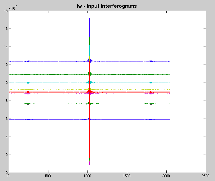
| Interferograms for 10 selected pixels across detector array:
|
|
|
|
|
|
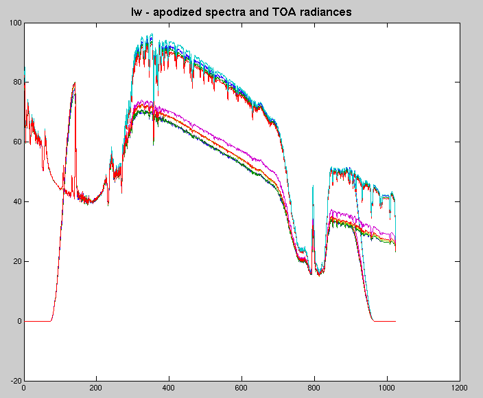
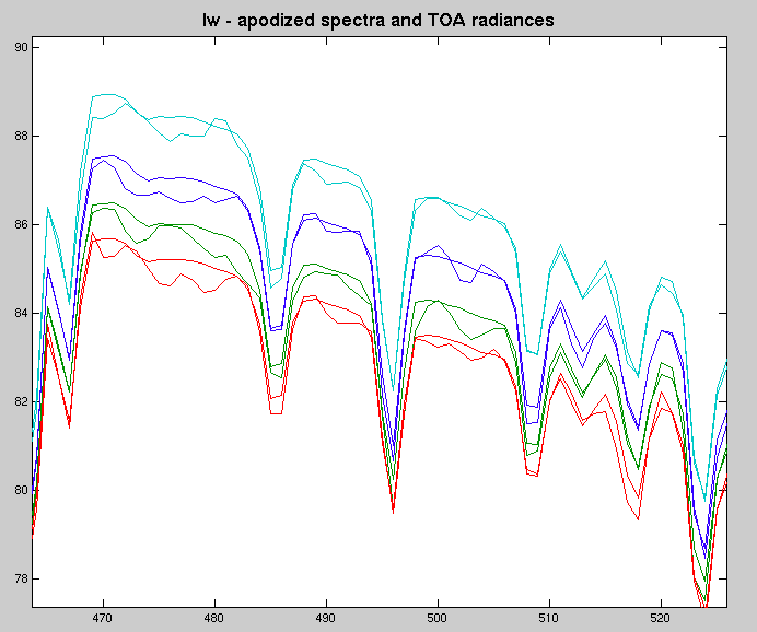
| TOA radiances along with corresponding apodized GIPS output for the above pixels:
|
|
|
|
|
|
| Closeup of the above - TOA rad and apodized GIPS output are colored by pixel:
|
|
|
|
|
|
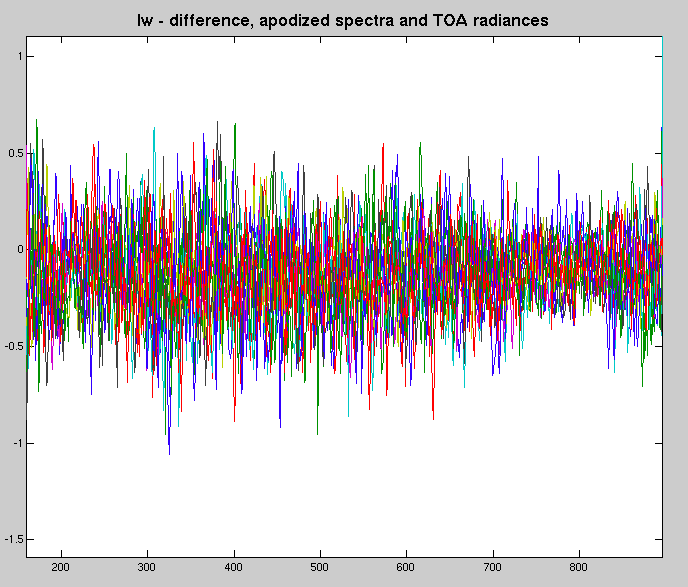
| difference betwee TOA radiances and GIPS output (apodized) for the above pixels:
|
|
|
|
|
|
 | Cube cross-sections of diff between TOA radiances and apodized GIPS outputs, in the Ozone spike region:
|
|
|
|
|
|
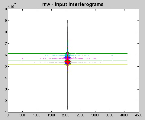
| Interferograms for 10 selected pixels across the MWIR detector array:
|
|
|
|
|
|
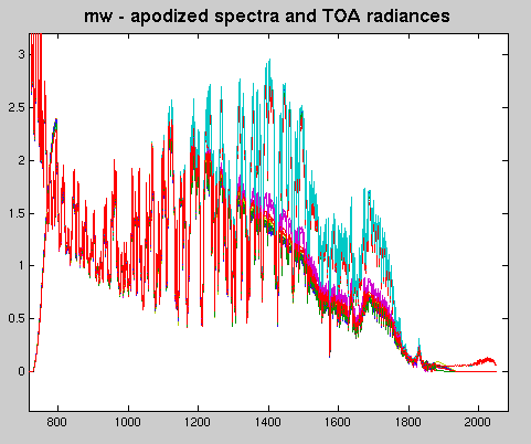
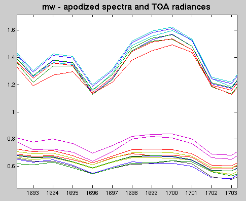
| plot of TOA Radiances and corresponding apodized GIPS outputs for same set of pixels:
|
|
|
|
|
|
| Closeup of the above: again, matching TOA radiances and GIPS apodized outputs have same color
|
|
|
|
|
|
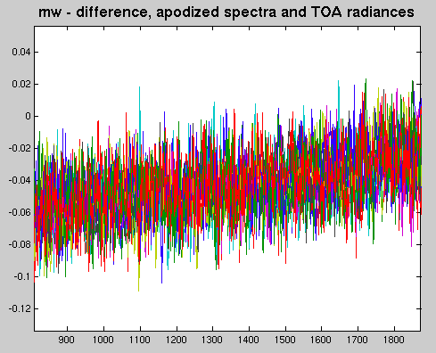
| The most interesting graph of this entire test report: a diff plot between TOA radiances and GIPS apodized output for the above pixels:
|
|
|
|
|
|
| note the overall tilt in the GIPS output!
|
|
|
|
|
|
| Plot of GIPS apodized output, cross section of single wavenumber for whole cube:
|
|
|
|
|
|
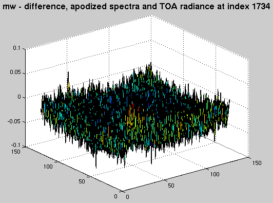
| diff of GIPS apodized output with TOA radiances for same wavenumber:
|
|
|
|
|
|
| When processing reasonable data, GIPS produces overall good output.
|
|
|
|
|
|
| a flat bias in the LW band and a tilt bias in the MW band will need to be investigated and corrected in future versions of GIPS
|
|
|
|
|
|
| the "mexican hat effect" introduced by optical system and sensor geometry is mostly but not entirely removed, proving the efficacy of the correction application procedure, but demonstrating the need for a better spectral calibration algorithm.
|
|
|
|
|