Animations of visible/IR imagery can be viewed by clicking on the desired date in the Table 1. Images are available from the GOES-10 sounder at 1 hour intervals. Visible images (band 19) are shown during daylight hours and window channel infrared images (band 8) are shown at night. Note that the 09 UTC image is unavailable on each day. Data from 16-18 April are unavailable at this time.
Table 1
|
|
|
|
|
|
|
|
|
|
|
|
|
|
|
|
|
|
|
|
|
|
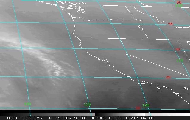
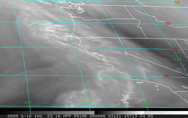
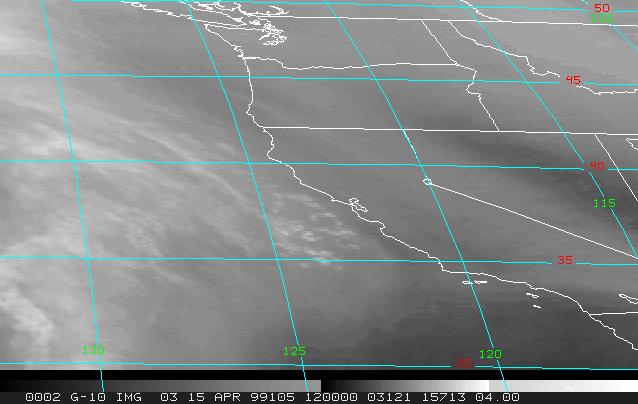
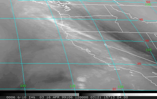
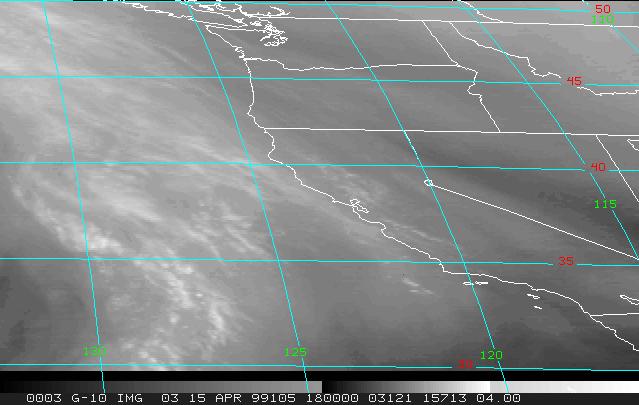
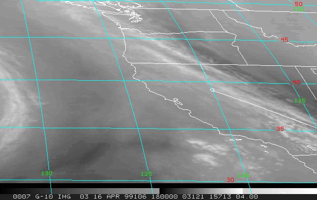
The evolution of fog off the
California coast can also be followed by comparing the visible imagery
at 00 and 16 UTC on 12-13 April ( fig.
1 ) and on 14-15 April ( fig.
2 ). The evolution of cloud cover on 09-10 April can also be viewed
in Fig.3 and Fig.4
.
Fields of Total Precipitable Water (TPW) and surface wind speed (SWS) are courtesy of Frank Wentz. The digital files for the images shown here were obtained from the Remote Sensing Systems SSM/I Web page and converted to McIDAS files. Data from 3 satellites are available for this time period (F11, F13, F14). The overpass times for each satellite are similar for each satellite, 03 and 15 UTC plus or minus 1-2 hours. The exact times of the data are available as images if needed (but are note shown here). Since there are gaps in coverage between each pass and occasional missing data, the data from all 3 satellites have been combined into single images twice a day and correspond to approximately to 03 and 15 UTC. Where overlapping data existed from more than 1 satellite, data are shown from F14 (in the case of F14 and F13 or F11) and F13 (in the case of F13 and F11). This priority was chosen arbitrarily. Perhaps it would be better to take an average, but it's my impression that the results will not differ significantly. Retrieved quantities can not be obtained over land due to high surface emission there. Missing data over water is indicated as white. This occurs in heavy precipitation, near coasts where contamination of emission from land is significant, and where data was not collected (transmission problems?).
To view images, just click on the X for the desired parameter and time in Table 2. For 10-15 April TPW, a sequence of the following images are shown:
1) SSM/I TPW,
2) GOES-10 TPW,
3) GOES Sounder, Band 10 (7.4 micron),
4) GOES Sounder, Band 11 (7.0 micron),
5) GOES Sounder, Band 12 (6.5 micron),
6) GOES Visible.
Sounder derived PW (mm) in low, middle and upper layers can be overlayed by clicking on the desired boxes: PW1, PW2, PW3, (corresponding to sigma layers 1.0-.9, .9-.7, and .7-.30 ,respectively). For the images of sounder bands 10-12, relatively dry (dark) and moist (bright) areas can be followed. The radiation in these bands is sensitive to temperature and water vapor in the low/mid to upper troposphere with broad weighting functions which peak at approximately 700, 500, 300 mb, respectively (for example, click here ). The heights of these weighting functions are not fixed, but vary with the atmospheric moisture profile itself. (For example. the weighting functions lower toward the surface as the atmosphere becomes drier).
Table 2
|
|
|
|
|
|
|
|
|
|
|
|
|
|
|
|
|
|
|
|
|
|
|
|
|
|
|
|
|
|
|
|
|
|
|
|
|
|
|
|
|
|
|
|
To view animations (movies) of the SSM/I SWS and TPW, click on the links below. Note that to animate the full time period requires the download of 36 images. It may take a while before the movie is set up and ready to run, depending on network speed & the amount of memory available to your computer. If the full time period takes too long (or doesn't complete), you may find it more practical to look at the first and second half of the time period separately. The movie can be toggled between SWS and TPW by clicking on the box marked "TPW". The movie uses a Java Applet written by Tom Whittaker at the Cooperative Institute for Meteorological Satellite Studies ( CIMSS ) at the University of Wisconsin-Madison.
To view an animation of derived cloud top properties from the GOES-10 imager, click on the link below.
The albedo at the near IR wavelength of 3.9 microns
is shown during the daytime (18 and 00 UTC image times). This albedo is
estimated from emitted radiation at 10.7 microns (band 4) and the reflected+emitted
radiation at 3.9 microns (band 2). The more highly reflective clouds are
enhanced in green (albedo > .20). These are stratus/fog clouds which have
low bases and consist of water droplets. Cloud tops composed of ice crystals
generally have lower albedos (< .10) at this wavelength. These are enhanced
as black or a dark shade of gray in the images. The albedo images can be
compared to the 4 km resolution visible images by stopping the loop and
clicking on the box marked "VIS/IR".
At night (06 and 12 UTC), the stratus/fog clouds
can be discriminated by subtracting the brightness temperature at 3.9 from
that at 10.7 microns. The result will be greater than zero for clouds composed
of small water droplets. This is because these clouds have a lower emissivity
and brightness temperature at 3.9 microns than at 10.7 microns. The areas
where the temperature difference is positive are highlighted in green.
For ice cloud tops and most land surfaces, the difference is nearly zero
or slightly negative. These appear as gray to white in the images. Thin
or broken ice clouds, such as cirrus, have a larger negative difference
and appear darkest in the images. This is because of the higher sensitivity
to sub-pixel warm spots at 3.9 microns where there is penetration of radiation
from the warmer earth surface below through the clouds. The temperature
difference images in this loop can be compared to the 10.7 micron (band
4) images by stopping the loop and clicking on the box marked "VIS/IR".
Note how difficult it is to distinguish the cloud cover from the sea surface
on the basis of the brightness temperature at 10.7 microns alone, as compared
to the 10.7-3.9 micron difference fields.
To view images showing cloud top temperatures and
derived cloud top pressures from 12-14 April, click here
.
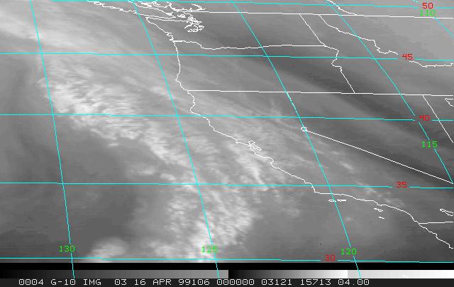
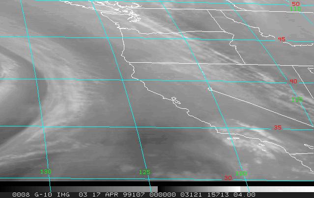
Inferring Subsidence from Water Vapor Imagery
Table
3 contains water vapor images (6.7 micron) from the GOES-10 imager. The
darkness of the images is proportional to
the equivalent black body temperature (BT). These
temperatures are indicated in degrees C at a few locations in the images.
The BT is inversely related to the mean relative humidity in the middle
and upper troposphere. In other words, warmer areas are drier. Subsidence
is likely where BT increases with time in the frame of reference of the
moving air. Note the formation of warming and cooling regions
around the upper low as it moves southeast along
the west coast on 11-12 April. As this system moves inland and weakens,
a nearly linear band of warming develops off the California coast between
00 and 06 UTC on 13 April. This is near the area where widespread stratus
develop. The band continues to intensify as it
moves south.
Table 3
|
|
|
|
|
|
|
|
|
|
|
|
|
|
|
|
|
|
|
|
|
|
|
|
|
|
|
|
|
|
|
|
|
|
|
|
|
|
|
|
|
|
|
|
These images can be animated by clicking here . In addition, hourly imagery from the 3 water vapor sounder bands (10,11,12) can be looped for 13 April by clicking the entries in Table 4. As discussed above Table 2, the radiation in these bands is sensitive to temperature and water vapor in the low/mid to upper troposphere with broad weighting functions which peak at approximately 700, 500, 300 mb, respectively (for example, click here ).
Table 4
|
|
|
|
|
|
|
|
|