|
McIDAS-V User's GuideVersion |
McIDAS-V is a free, open source, visualization and data analysis software package that is the next generation in SSEC's 40 year history of sophisticated McIDAS software packages. McIDAS-V displays weather satellite (including hyperspectral) and other geophysical data in 2- and 3-dimensions. McIDAS-V can also analyze and manipulate the data with its powerful mathematical functions. McIDAS-V is built on SSEC's VisAD and Unidata's IDV libraries, and contains "Bridge" software that enables McIDAS-X users to run their commands and tasks in the McIDAS-V environment, and an integrated version of SSEC's HYDRA software package.
This McIDAS-V User's Guide is currently under construction. Once completed, it will describe using the features available in the McIDAS-V application. For a brief description about getting started using McIDAS-V and making displays of common data available, refer to the Getting Started section.
This Guide was originally developed at the Unidata Program Center by the developers of the Integrated Data Viewer (IDV). The first version of the McIDAS-V User's Guide was created from the IDV User's Guide (September 2007) and has since been updated to reflect the changes that have been made to McIDAS-V, IDV, and VisAD (see the Release Notes for details on recent changes).
Development of McIDAS-V is ongoing at the Space Science and Engineering Center (SSEC) at the University of Wisconsin-Madison. The development is driven by the needs of the community of users. Suggestions, comments, and collaboration are welcomed and encouraged. See Documentation and Support for more information. The goal is to provide new and innovative ways of displaying and analyzing Earth science data, as well as provide common displays that many of its users have come to expect.
See Downloading and Running McIDAS-V for information on how to download McIDAS-V, install McIDAS-V, and run McIDAS-V. For additional information, refer to the latest McIDAS-V training materials.
The items below list the changes in McIDAS-V for the most recent released versions.
For a current list of known bugs and requested enhancements, please see the Open Inquiries Report from the McIDAS-V Inquiry System. To view the items currently under development, see the list of Critical Bugs and Critical Development Items.
The items below reflect the changes since the 1.3 release.
Continued to add to the suite of fully supported Jython scripting tools introduced in McIDAS-V 1.2. The functions and methods in this suite can be used to load and display data, manipulate the display, and save the images. This allows the user to automatically process data and generate displays for web pages and other environments. This scripting can be done from the Jython shell within McIDAS-V, or from a Jython script that can be invoked as a command line argument. Please see Scripting for the list of supported functions, an example script, and links to various Java docs.
Since the release of McIDAS-V 1.3, there are new functions designed to work with ADDE data. These functions are:
makeLocalADDEEntry - Creates a local ADDE entry in the server table.
getLocalADDEEntry - Gets the descriptor for a local ADDE Entry.
listADDEImages - Lists data from an ADDE image server.
listADDEImageTimes - Lists available dates and times of data from an image server.
There is also a new version of getADDEImage that gives different output than the previous version.
Changed the Save Data window when saving a zipped bundle to make it easier to determine what data will get saved with your bundle. This is now done through radio buttons.
Reformatted the Layer Controls for the RGB Composite display. There is now an Apply button that will apply any changes to the red, green or blue minimum, maximum, or gamma values directly to the display without having to press Enter. There is also now an Apply to All Gamma Fields button that will apply a common gamma value to all colors.
Added the ability to set logging level in the Advanced tab of the User Preferences window. The logging level you select will determine how much information gets written out to your mcidasv.log file in your McIDAS-V directory. For more information about each of the logging levels and what they entail, please see the Log Level section of the Advanced Preferences page.
Reworked the Formula Editor to make it more intuitive to users. The Description field has moved out of the Advanced section of the Formula Editor, and into the top main section. The value in the Description field will be what is written out in the Field Selector as the name of the formula. The Name field of the Formula Editor has changed its name to ID, and is used when setting Parameter Defaults.
Added the ability to work with Suomi NPP data from NOAA CLASS that includes the data and geolocation within the same file. Non-consecutive granules can now be displayed, and granules can now be aggregated regardless of granule size. VIIRS SVI data from CLASS can now be displayed. Saving of both zipped and unzipped bundles containing NPP data is now supported.
There has been added functionality for working with VIIRS Cloud Mask products. If a GMODO-IICMO* product is loaded, there are various quality flag products included with the data. McIDAS-V now has the ability to determine which quality flag products are included with the data as well as what cloud mask fields can be produced from them. With cloud mask products, fields such as 'Cloud Phase', 'Volcanic Ash', 'Dust' and 'Fire' can be displayed.
There has been added functionality for working with VIIRS EDR (Environmental Data Records) products. These products include fields such as cloud heights, pressures, and temperatures, sea surface temperatures, and snow cover.
This is currently located in the Under Development list of choosers in the Data Sources tab of the Data Explorer and is available for user feedback through the McIDAS-V Support Forums. As the IDPS (Interface Data Processing Segment) begins to distribute new types of NPP data, we test it in McIDAS-V and make any necessary changes to be able to get the data to display.
The items below reflect the changes since the 1.2 release.
Updated all local ADDE image servers, except for MODIS, to the versions included in McIDAS-X 2013.1. The most significant enhancements were updates to the Meteosat server (to include calibration updates, support Meteosat-10 data, and support MSG compressed and rapid scan data) and the NOAA/Metop AVHRR Level 1b server (to support Metop-B data and pre-KLM series NOAA POES data).
A new version of the netCDF-Java library (4.3.16) is included in this release. This version of netCDF-Java includes major changes to the way GRIB 1 and 2 files are handled. See the netCDF-Java GRIB documentation for a more details on these changes.
One major outcome of this change is that GRIB variable names will now be generated in a very general way. This means that bundles that were generated with a previous version of McIDAS-V might break. In order to aid users in the transition between netCDF-Java 4.2 and 4.3, the netCDF-Java library has provided a mapping of old variable names and new variable names for the datasets served on the Unidata THREDDS Data Server (TDS), and this mapping is being used 'under the hood' in McIDAS-V to minimize the impact of these changes on users.
For users reading GRIB files from other locations (local files or other remote servers), McIDAS-V now allows users to make custom variable name mappings. New variable mappings should be placed in the McIDAS-V/varrenamer.xml file. The structure of this file is quite simple:
<varrenamers>
<varrenamer
old="oldNameHere"
new="newNameHere" />
<varrenamer
old="anotherOldNameHere"
new="anotherNewNameHere" />
</varrenamers>
Changes to the way GRIB files are served via the Unidata TDS server have also been made. The impact of this change is that the dataset URLs that point to GRIB resources will change, which will break bundles that point to the old Unidata TDS (motherlode.ucar.edu).
Again, in order to aid users in this transition, the netCDF-Java library has provided a mapping between the old and new dataset URL paths for all datasets served through the Unidata TDS. As with the variable name changes, the URL mapping for datasets on the Unidata TDS is being used 'under the hood' in McIDAS-V to minimize the impact on users.
The latest version of TDS (4.3), where URL related impacts will be seen, is now running on the main Unidata TDS (thredds.ucar.edu). Starting with version 1.3, McIDAS-V will redirect all requests to the old Unidata TDS (motherlode.ucar.edu) to the new Unidata TDS (thredds.ucar.edu) automatically and update the appropriate data URLs.
As TDS servers in the community begin to upgrade to TDS 4.3, users will likely need to use custom URL mappings. New URL mappings should be placed in the McIDAS-V/urlmaps.xml file.
Again, the format of this file is quite simple:
<urlmaps>
<urlmap
type="opendap"
old="oldthreddsserver1.edu/"
new="newthreddsserver1.edu/" />
<urlmap
type="opendap"
old="threddsserver2.edu/thredds/dodsC/old/path/"
new="threddsserver2.edu/thredds/dodcC/new/path/" />
</urlmaps>
In the first example, a new THREDDS server has replaced an old server - all requests going to oldthreddsserver1.edu will be directed to newthreddsserver1.edu. The second example is where the URL path to a particular dataset has changed, either because the product has been replaced (for example, the RUC to the RAP transition) or the maintainer of the TDS server has changed the way data are cataloged. Note in both cases the type of URL is an opendap URL. In the future, this mechanism will be used to redirect other types of data requests.
Added the ability to work with Suomi NPP data from NOAA CLASS that includes the data and geolocation within the same file. You can now display non-consecutive granules. You can also now aggregate granules together regardless of granule size. VIIRS SVI data from CLASS can now be displayed. Saving of both zipped and unzipped bundles containing NPP data is now supported.
There has been added functionality for working with VIIRS Cloud Mask products as well. If you load in a GMODO-IICMO* product, there are various quality flag products included with the data. McIDAS-V now has the ability to determine which quality flag products are included with the data as well as what cloud mask fields can be produced from them. Therefore, if you load in a GMODO-IICMO* file, you will see fields such as 'Cloud Phase', 'Volcanic Ash', 'Dust', 'Fire', etc.
This is currently located in the Under Development list of choosers in the Data Sources tab of the Data Explorer and is available for user feedback through the McIDAS-V Support Forums. As the IDPS (Interface Data Processing Segment) begins to distribute new types of NPP data, we test it in McIDAS-V and make any necessary changes to be able to get the data to display.
The items below reflect the changes since the 1.01 release.
The items below reflect changes since the 1.0 release.
You can use the Grid->Define a grid diagnostic formula to use these functions.
Redesigned the Satellite Imagery Chooser to include new options, such as an optional preview image in the Region tab of the Field Selector.
Users are encouraged to use this new chooser. Please notify us (via the McIDAS-V Support Forums or McIDAS Help Desk) if you feel there is something in the previous chooser that should be implemented in the new chooser. The previous chooser is available through the Legacy Choosers tree.
McIDAS-V should run on any platform that fully supports Java and Java 3D. It has been tested on Linux, Mac OS X, and Windows. AIX and IRIX support the requirements in certain configurations, but have not been tested.
To run McIDAS-V, a system will need to have a minimum of a 500 MHz processor and 512 MB of RAM free. However, if you are purchasing a new system, it is recommended that an Intel system running McIDAS-V have at least a 2 GHz processor and 4 GB memory (RAM). Please note that Java on 32 bit operating systems can only utilize 1536 MB, while 64 bit operating systems can utilize all of the available memory. Performance will be better with faster processors and more memory. We have seen the best results with NVIDIA hardware and drivers.
Detailed requirements for the following are listed below:
The chart below lists the software versions, by vendor, that McIDAS-V is known to run on, and that McIDAS User Services tests:
OS |
Known to Work |
Tested at SSEC (1) |
|---|---|---|
| Linux | Red Hat Linux 4.0+ |
Red Hat Enterprise Linux WS 5.7 (32 bit) Red Hat Enterprise Linux WS 6.1 (64 bit) |
| Mac OS X(2) | Mac OS X 10.6+ | Mac OS X 10.6 Mac OS X 10.7 Mac OS X 10.8 |
| Windows | Windows XP, Vista, 7 | Windows XP with Service Pack 3 Windows Vista with Service Pack 2 Windows 7 Enterprise |
Notes:
(1)The local ADDE servers are distributed as binaries compiled only on these Operating System versions. If you are running versions other than those listed, the local ADDE servers may not work and give you an error message that the "Local Server is not running".
(2)Due to changes in the requirements of the netCDF package, McIDAS-V requires Java 1.6. Some Mac OS X systems do not support Java 1.6 and thus are unable to run McIDAS-V. These include:
- All with PPC processors
- Intel Core Solo and Core Duo running OS X 10.5 or earlier
McIDAS-V works on systems with graphics cards that support OpenGL (all systems) and Direct-X (version 8.0+, Windows only). On Linux, the driver must support GLX, an X windows system extension to OpenGL programs. McIDAS-V also works on systems with stereo graphics cards. We have seen the best results with NVIDIA hardware and drivers, and with the display configuration set to a high screen resolution and the maximum number of colors.
McIDAS-V utilizes the latest developments in graphics cards, drivers and Java3D. If you encounter any problems with system instability (such as using all of the memory or CPU on your machine, or frequent software crashes) or unusual data displays with "torn" or "gray" images, you should make sure you have the latest driver for your system. Even if the system is brand new, the driver may not be the most recent version available.
Please Note: We have received reports of McIDAS-V failing to start (i.e., the windows never appear) on some systems using integrated graphics chipsets, including:
- Intel GMA 4500MHD
- Intel GM965
- ATI Radeon X300 family (including X550, X1050 and R300)
To determine the brand and driver information of your graphics card, follow the guides for each platform below:
Once you have determined your graphics card brand and driver information, check the manufacturers web page for information on their updated versions. Here are links to some of the most common graphic card Original Equipment Manufacturers (OEM):
McIDAS-V is packaged with the following versions included:
Versions Included with McIDAS-V |
|||
|---|---|---|---|
JRE (Java Runtime Environment) |
Java3D |
JOGL (Java OpenGL) |
|
| Linux(1) | 1.6.0 |
1.5.2 |
n/a |
| Mac OS X | included with Mac OS X(2) |
1.5.2 |
1.1.1 |
| Windows(3) | 1.6.0 |
1.5.2 |
n/a |
| other unix | none |
none |
n/a |
The necessary versions of the JRE, Java3D and JOGL are included with the Linux, Mac OS X, and Windows installers. On other platforms, you will need to install Java and Java3D before installing McIDAS-V. If other platforms fully support Java version 1.6+ and Java 3D version 1.3.1+ (e.g. AIX, IRIX), they should also work, but have not been tested.
Notes:
(1)The version of the Mesa library that comes with Red Hat Linux may be incompatible with Java 3D packaged with McIDAS-V. If you experience X server crashes when exiting McIDAS-V, you will need to build and install Mesa from source available at http://www.mesa3d.org.
(2)To find and/or update your default Java version, follow these steps:(3)You must have DirectX version 8.0+ installed on your Windows system if you use the DirectX rendering mode of Java 3D (the default is to use OpenGL).
- Open the "Java Preferences" application located in /Applications/Utilities
- Look for "Java SE 6" in the "Java Applications" section
- The version at the top of the "Java Applications" list is the version being used by McIDAS-V. If "Java SE 6" is not at the top of the list, click and drag it to the top of the list (using the 64-bit option, if available). If "Java SE 6" is not in the "Java Applications" list, you may need to manually run the Software Update feature in the Apple Menu.
McIDAS-V can be demanding of hardware speed and memory depending on the size of the datasets you wish to work with. It is recommended that the system have a minimum of 512 MB of RAM free for McIDAS-V use. Performance is significantly better with 1 GB RAM or more. Please note that 32 bit Java Runtime Environments (JRE) can utilize a maximum of 1536 MB RAM, while 64 bit JREs can utilize all of the RAM available to the operating system (64 bit OS required).
The recommended processor speed will vary by platform. You can run on a system as slow as 500 MHz or even less, but response will be correspondingly reduced. In general, the faster the processor, and the more memory your system has, the better the performance will be.
For reasonable performance, it is recommended that an Intel system running McIDAS-V have at least a 2 GHz processor and 4 GB memory (RAM). Performance will be even better with faster processors and more memory.
McIDAS-V is designed to access data on remote servers on the Internet, as well as from local files. Downloading data from remote servers benefits from a fast connection to the Internet, since many data fields are large.
This page contains information on:
If you have any trouble downloading and installing McIDAS-V, first check the FAQ, then please report your problem as described in McIDAS-V Support.
For more information on downloading and using McIDAS-V, please see the Installation and Introduction tutorial on the McIDAS-V Documentation Page. Also, see this page for additional tutorials and instructional videos on more advanced subjects.
Check that your system meets the System Requirements for McIDAS-V and download the appropriate package for the following operating systems:This file is just the installer and can be placed anywhere on your machine. When you run the installer in the next step, you can then indicate where you want McIDAS-V to be installed.
Start the installer by following the instructions appropriate for your operating system:
|
|
|
|
|
|
|
|
A GUI will walk you through the installation steps and allow you to create a program group and/or desktop icon. When McIDAS-V is installed, a McIDAS-V-System directory will be created in your installation directory. This directory contains system files necessary to run McIDAS-V and users should not save files to the McIDAS-V-System directory.
Note: Windows users should not install McIDAS-V in the /Program Files directory as this can lead to permissions problems.
If an error occurs, please see the FAQ for information on solutions to common errors reported by users installing and running McIDAS-V. If you do not see your error listed, please send a support request to McIDAS-V Support.
On Mac OS X:
Double-click on the McIDAS-V shortcut icon that was created in /Applications.
Double-click on the McIDAS-V shortcut icon that was created on the Desktop.
At the UNIX prompt from the directory where McIDAS-V was installed, run the command: McIDAS-V-System/runMcV.
If an error occurs, please see the FAQ for information on solutions to common errors reported by users installing and running McIDAS-V. If you do not see your error listed, send a support request to McIDAS-V Support or use the Support Request Form in the Help menu of McIDAS-V.
Note: When McIDAS-V is first run, a /McIDAS-V directory will be created in the user path. This directory contains information about user-specified settings as well as XML files for color tables, projections, etc. that are used by McIDAS-V. Users can write files to this directory.
McIDAS-X users who install McIDAS-V and want to run their McIDAS-X commands in the McIDAS-V environment via the Bridge must also be running McIDAS-X on the same computer. Sites that have joined the McIDAS Users' Group and purchased McIDAS-X support can download the current version of McIDAS-X from the McIDAS-X Downloads page.
By default, McIDAS-V uses 80% of the available memory on your machine. The maximum amount of memory is determined by the operating system. To manually change the amount of memory used by McIDAS-V, edit the Maximum Heap Size in the Advanced tab of the Preferences by selecting Edit->Preferences... from the main menu. The new amount of memory will be saved and used in subsequent sessions. For 32 bit operating systems, it is recommended to set this to no more than 1250 MB. The maximum value for 32 bit operating systems is 1536 MB, while 64 bit operating systems can use all of the RAM available. To change the amount of memory used to a percentage, select the percentage option in the Advanced tab of the User Preferences by selecting Edit->Preferences... from the Main Display window.
The source code for McIDAS-V is available for download. For instructions on building McIDAS-V from source, see the Building McIDAS-V from Source document.
McIDAS-V can read a variety of data formats either from local files or remote data servers (e.g., HTTP, TDS, ADDE). This page contains information about some data sources that work with McIDAS-V.
To connect McIDAS-V to data sources, see Data Sources.
| Data Type | Description | Supported Formats | Access Method |
|---|---|---|---|
| Gridded | Numerical weather prediction models, climate analysis, gridded oceanographic datasets, NCEP/NCAR Reanalysis | - netCDF | - local files, HTTP, TDS servers |
| - GRIB (versions 1&2) | - local files, TDS servers | ||
| - Vis5D | - local files, HTTP | ||
| - GEMPAK | - local files, TDS servers | ||
| Satellite Imagery | Geostationary and polar orbiter satellite imagery, derived satellite products | - ADDE | - ADDE servers |
| - McIDAS AREA | - local files, local & remote ADDE servers | ||
| - AIRS | - local files | ||
| - GINI | - local files, TDS servers | ||
| - AMSR-E Level 1b | - local ADDE | ||
| - EUMETCast LRIT | - local ADDE | ||
| - Meteosat OpenMTP | - local ADDE | ||
| - Meteosat Second Generation (MSG) Level 1b | - local ADDE | ||
| - Metop AVHRR Level 1b | - local ADDE | ||
| - MODIS L1b MOD02 (MODIS Level 1b) | - local ADDE | ||
| - MODIS L2 MOD04 (Level 2 Aerosol) | - local ADDE | ||
| - MODIS L2 MOD06 (Level 2 Cloud Top Properties) | - local ADDE | ||
| - MODIS L2 MOD07 (Level 2 Atmospheric Profile) | - local ADDE | ||
| - MODIS L2 MOD28 (Level 2 Sea Surface Temperature Products) | - local ADDE | ||
| - MODIS L2 MOD35 (Level 2 Cloud Mask) | - local ADDE | ||
| - MODIS L2 MODR (Level 2 Corrected Reflectance) | - local ADDE | ||
| - MSG HRIT FD and HRV | - local ADDE | ||
| - MTSAT HRIT | - local ADDE | ||
| - NOAA AVHRR Level 1b | - local ADDE | ||
| - SSMI (TeraScan netCDF) | - local ADDE | ||
| - TRMM (TeraScan netCDF) | - local ADDE | ||
| Radar | Radar images | - Level II | - local files or TDS (bzip2 compressed or uncompressed) |
| - Level III | - ADDE servers, local files or TDS | ||
| - Universal Format (UF) | - local files | ||
| - DORADE | - local files | ||
| Point Observational | Surface observations (METAR and SYNOP), earthquake observations | - ADDE | - ADDE servers |
| - netCDF (Unidata, AWIPS/MADIS formats) | - local files | ||
| - Text (ASCII, CSV), Excel spreadsheet | - local files | ||
| Aircraft observations | - netCDF (RAF convention) | - local files | |
| - Text (ASCII, CSV) | - local files | ||
| Global balloon soundings | - ADDE | - ADDE servers | |
| - netCDF (Unidata, AWIPS/MADIS formats) | - local files | ||
| - CMA text format | - local files | ||
| Profiler | NOAA Profiler Network winds | - ADDE | - ADDE servers |
| GIS | Data typically used in Geographic Information Systems (GIS) | - ESRI Shapefile | - local files, HTTP |
| - USGS DEM | - local files | ||
| QuickTime | QuickTime movies (without extensions) | - QuickTime | - local files, HTTP |
Extensive meteorological and oceanographic data is available from remote data servers for use in research and education. Some of these data have restrictions on their use, see Using Data Acquired via Unidata for that information.
Most of the data choosers in McIDAS-V use ADDE as the access method (satellite imagery, Level III radar, surface, profiler and RAOB). The ADDE choosers are pre-configured with a list of available servers. SSEC and the Unidata community each maintain a set of cooperating ADDE servers which serve up real-time and archived atmospheric datasets for use in McIDAS-V. You can use any of these to access the near-realtime data. For more information on accessing data on ADDE servers, see the Data Sources section.
SSEC image data sets include:
Additional image data sets:
You can configure defaults for particular images by creating a custom defaults file. For more information, see Configuring Image Defaults.
*Additional alternate servers include: idd.unl.edu, stratus.al.noaa.gov, twister.millersville.edu, weather2.admin.niu.edu, and weather3.admin.niu.edu. These alternate servers have most or all of the datasets listed under adde.ucar.edu.
McIDAS-V can access gridded data (netCDF/GRIB/GEMPAK) and NEXRAD radar data stored on a THREDDS Data Server (TDS) through the OPeNDAP (formerly called DODS) protocol. See Choosing Cataloged Data for more information.
Many of the data sources listed in the table above can read files directly from web servers (e.g. Apache) through the HTTP protocol. In most cases, the server must support the HTTP 1.1 protocol and be configured to set the "Content-Length" and "Accept-Ranges: bytes" headers. See the Choosing a URL for more information.
The Network Common Data Form (netCDF) provides a common data access method for Unidata applications. This format can be used to store a variety of data types that encompass single-point observations, time series, regular grids, and satellite and radar images. The mere use of netCDF by itself is not sufficient to make data "self-describing" and meaningful to McIDAS-V.
Generally, McIDAS-V requires that datasets in netCDF format use metadata conventions to be able to fully understand and geolocate the dataset. These conventions provide documented "best practices". Using conventions with netCDF ensures your data is complete and self-describing, and can be used by others. We recommend you use CF, COARDS, or NUWG conventions for netCDF data files for McIDAS-V, and be sure to follow the best practices noted above.
McIDAS-V can read point data and trajectories (aircraft tracks) from comma-separated value (CSV) text files. See the documentation on the Text (ASCII) Point Data Format.
The first source of support is this McIDAS-V User's Guide. It contains complete instructions for downloading, installing, running, and using the McIDAS-V reference application and all its features. It also has a Frequently Asked Questions (FAQ) section with answers to many of the most commonly asked questions. The User's Guide can be accessed from the McIDAS-V Help->User's Guide menu or online at https://www.ssec.wisc.edu/mcidas/doc/mcv_guide/current/.
Additional documentation is available on the McIDAS-V homepage (https://www.ssec.wisc.edu/mcidas/software/v/), including McIDAS-V training materials (tutorials and data used in training sessions) and McIDAS-V source code.
If you have questions or encounter problems that the McIDAS-V documentation (described above) doesn't provide sufficient help, there are two additional sources of help. They are the McIDAS-V Support Forums and the McIDAS Help Desk.
The McIDAS-V Support Forums contain subject-based forums, each with topics and posts relating to the forum's subject. Only registered users can post on the forums. However, anyone can view the forums and their contents (i.e., visit as an unregistered "Guest").
The McIDAS Help Desk is staffed during business hours with user-support personnel. As noted in the MUG Policy Document, the help desk is supported by the fees paid by the McIDAS Users' Group (MUG) and thus provides advanced-level support for MUG members. For McIDAS-V all users (whether or not a MUG member) are welcome to contact the help desk to report software bugs or suggest improvements (enhancements).
When reporting a bug, first check for related error messages in the Message Console, and include the appropriate error messages in your email message. Also include as much information as you can about how you were running McIDAS-V and what happened, including:
Send this information to the McIDAS Help Desk using one of the three methods below.
McIDAS User Services
Space Science and Engineering Center
University of Wisconsin-Madison
1225 West Dayton Street
Madison, WI 53706
McIDAS-V includes software developed by:
Please read the different LICENSE files present in the root directory of the McIDAS-V distribution for restrictions on those packages.
This section describes how to quickly get started using McIDAS-V and making displays of common data.
There are two main windows in the McIDAS-V application, the Data Explorer window and the Main Display window. Other windows may appear when needed.
The Data Explorer window is central to McIDAS-V. It is used to choose data sources and parameters to display, the types of displays to make, and times of data to display. More information can be found in the Data Explorer section of the McIDAS-V User's Guide.
The Main Display window includes the McIDAS-V display panels, Legend, Time Animation Controls, viewpoint controls for 3D displays, icons for zooming, panning, and rotating, menus of projections, the main McIDAS-V toolbar, and the main menu bar. More information can be found in Main Display window section of the McIDAS-V User's Guide.
To create displays with McIDAS-V, the common usage scenario is:
For more help with getting started with McIDAS-V, please see the Installation and Introduction tutorial on the McIDAS-V Documentation webpage.
This section describes how to make displays using geostationary and polar orbiting satellite imagery.
The steps include:
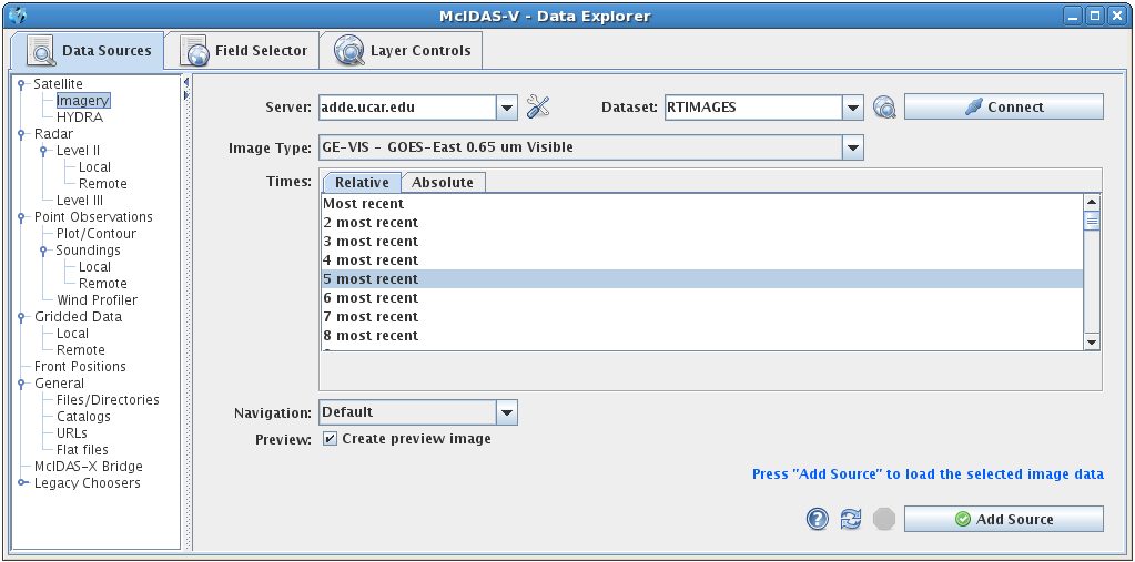
In the Data Explorer window, select the Data Sources tab. On the left side of this tab, select Satellite->Imagery from the list of available choosers. For more information about the imagery chooser, see Choosing Satellite Imagery.

McIDAS-V comes pre-configured with a list of ADDE servers and datasets, or you can enter your own. See Available data for a description of these pre-defined data sets.


When choosing absolute times for the first time McIDAS-V needs to query the ADDE server for the times. This may take some time. To select more than one time use Ctrl+click or Shift+click.

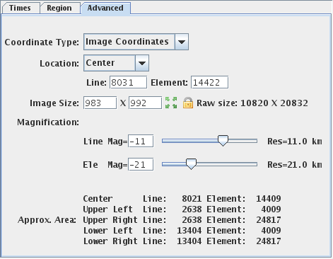
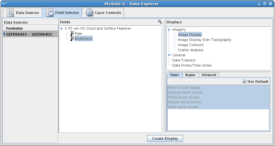
The image data source that you selected will be shown in the Field Selector tab. The available display types are listed in the Displays panel, the times are listed in the Times tab, the preview image or map is displayed in the Region tab, and the geographical selection parameters are listed in the Advanced tab.

If you want to create another type of satellite display over your current display, click "Image Contours" in the Displays panel to contour your data. To change your contour colors, right click on the color bar in the Legend, and choose one of the color tables shown in the list.
Due to the variability in brightness values in satellite images, some changes may need to be made to the contours to produce a quality image. To reduce the number of contours in the image, the contour interval can be increased by clicking the ![]() button next to Contour in the Layer Controls tab of the Data Explorer, and entering a higher value for the Contour Interval. To decrease the rigidness of the contours, select a new Smoothing method in the Layer Controls tab and enter a higher smoothing factor.
button next to Contour in the Layer Controls tab of the Data Explorer, and entering a higher value for the Contour Interval. To decrease the rigidness of the contours, select a new Smoothing method in the Layer Controls tab and enter a higher smoothing factor.
Return to the Satellite Imagery chooser in the Data Sources tab of the Data Explorer. Selecting polar orbiting satellite data is similar to the method to select geostationary data.
When creating loops of polar orbiting satellite images, it is recommended that the Auto-set Projection option be turned off, and a global projection be used in the map display to ensure all images can be viewed. For this example, turn the Auto-set Projection option off by going to the Main Display window and selecting Projections->Auto-set Projection. Under the same menu, change your projection to Projections->Predefined->World. These options can also be used for displaying single images of polar orbiting satellite data. If you have access to an ADDE server with Aqua or Terra granules, you can use the following steps to display the data:

This section describes how to create multispectral displays using HYDRA. The set of steps include:
In the Data Explorer window, select the Data Sources tab. On the left side of this tab, select Satellite->HYDRA from the list of available choosers. For more information about the HYDRA chooser, see Choosing Hyperspectral Data.
The HYDRA chooser is fairly similar to the File
Chooser. As a demonstration, download the IASI image from January 15, 2007 located at: ftp://ftp.ssec.wisc.edu/pub/mug/mcidas-v/training/data/IASI_xxx_1C_M02_20070115_1140.nc.
Navigate to the directory the file is in and press ![]() .
.
In the Field Selector tab of the Data Explorer, select Imagery->Multispectral Display, and click the ![]() button.
button.
There are four aspects to the multispectral display. The first is the image in the Main Display window. The image will be over Northern Africa and the Mediterranean Sea. The second aspect is the Spectra. The Spectra is displayed in the Layer Controls tab under "MultiSpectral". The spectra displayed by default is the 919.50 cm-1 spectral region (10.8 µm). The final two aspects are the two spectrum probes. In the Main Display window, there are two colored square boxes that represent the main probe (magenta) and the reference probe (light blue). These two probes are listed under "Readout" under "No Display" in the Layer Controls tab of the Data Explorer. Left click and drag either probe to view the spectra measured in various pixels around the image, or use one as a reference spectrum.
Change the wavenumber being displayed to 852.25 cm-1 by entering in the value into the Wavenumber: box in the Multispectral Display and hitting Enter. Move the magenta and light blue spectra probes to the approximate locations in the image below to locate an inversion at the location of the red box over Albania.
Once the two probes are in the approximate locations, the MultiSpectral window should look similar to the image below.
Zoom in over the 852.25 cm-1 region using the Ctrl+left click+drag combination to create a box of the region to zoom in on. If you miss the region, or want to return to the full spectra, use Shift+left click. The inversion should become clear as you zoom in, as shown in the image below.
For more help with displaying hyperspectral satellite imagery using HYDRA data, please see the Hyperspectral Data tutorial on the McIDAS-V Documentation webpage.
This section describes how to make displays using NWS WSR-88D Level II data. The steps include:
The Level II data is supplied as volume-scan files, each file having all data from WSR-88D radar for all sweeps for one "time". Archived Level II data is available from the National Climatic Data Center (NCDC) (data from NCDC must be un-tarred).
The files should be stored on your local file system with each station's files in a directory whose name is the 4-character ID (e.g., KTLX for Oklahoma City). In many cases, the data files do not have any location information in them and McIDAS-V uses the directory name as a first guess at the station location.
In the Data Sources tab of the Data Explorer, select Radar->Level II->Remote to view the Level II radar chooser. The Radar->Level II->Local chooser allows you to choose Level II data from your file system. For more information about the Level II radar chooser, see Choosing NEXRAD Level II Radar Data.
Select a station and a relative or absolute set of times. When done, click the ![]() button.
button.
The data source is shown in the Field Selector tab of the Data Explorer. Level II data has three moments or data types: Reflectivity, RadialVelocity, and SpectrumWidth. McIDAS-V has several display types for Level II data, and any of the moments can be shown with any of the displays. Selecting "Reflectivity" in the Fields panel will show the list of available displays in the Displays panel.
Select the Radar Sweep View in 2D under Radar Displays in
the Displays panel and click ![]() . Radar
Sweep View in 2D plots the data as a colored image on the base of
the 3D display area.
. Radar
Sweep View in 2D plots the data as a colored image on the base of
the 3D display area.
The Radar Sweep Controls allow you to change which sweep elevation you want to use. You can add range rings with the Displays->Add Range Rings menu item.
Select the Radar Sweep View in 3D entry under Radar Displays in the Displays panel. The Radar Sweep View in 3D display plots the data as a colored image, with the data plotted in 3D space at the elevation where the sweep occurred. You can rotate the display to see its 3D nature.
You can use this display to merge radar data displays with upper air data, such as McIDAS-V plots of NOAA Profiler data. Since the Earth is projected onto a flat surface in this display, the sweep has a shape very close to a rotated parabola. The Elevation Angles menu in the Layer Controls tab allows you to change which sweep elevation to display.
Select RHI (Range-Height Indicator) under Radar Displays in the Displays panel and press Create Display. The RHI display plots the data as a colored vertical cross section at the true elevations of the beams in 3D space (Image 5). This pseudo-RHI is constructed from several horizontal sweeps of the radar. It may be necessary to rotate the display to see the RHI in 3D.
The beam width is indicated by the vertical extent of each colored vertical stripe, corresponding to a bin beam bin sample. The position of the RHI in azimuth can be adjusted by dragging the little box on the end of the selector line above the RHI.
A 2D plot of pseudo-RHI (Image 6), is shown in the Display tab of the Layer Controls tab. The RHI displays have an auto-rotate feature and a Time Animation Widget.
Select Volume Scan (all sweeps) in the Displays panel in the Field Selector. Volume Scan (all sweeps) plots the data as 3D field of points colored by value. Each point is a bin value; all sweeps and bins are shown.
Select Radar Isosurface under Radar Displays in the Displays panel in the Field Selector tab. An isosurface is a 3D analog of a contour line which shows the location of all data with a single data value. Interpolation is used between sweep altitudes in the isosurface plot of Level II data, and all data in a volume scan is used.
To select Level II data from the Radar Imagery->Level II->Local file chooser:
For more help with displaying Level II radar imagery, please see the Level II Radar Imagery tutorial on the McIDAS-V Documentation webpage.
This section describes how to make displays using NWS WSR-88D Level III data.
The steps include:
In the Data Explorer window, select the Data Sources tab. On the left side of this tab, select Radar->Level III from the list of available choosers. For more information about the Level III radar chooser, see Choosing NEXRAD Level III Radar Data.


The Decluttter checkbox allows you to show all stations (not checked), or only a limited number of stations that do not overlap each other (checked). You will need to zoom in to see all the stations without overlaps.
When choosing absolute times for the first time McIDAS-V needs to query the ADDE server for the times. This may take some time. To select more than one time use Control+click or Shift+click.
The radar data source that you selected will be shown in the Field Selector tab of the Data Explorer.
Open up the Base Reflectivity tab under the Fields panel
(![]() ) to select
a data type. Select "Image display" in the Displays panel
under Imagery, and make the display by clicking the
) to select
a data type. Select "Image display" in the Displays panel
under Imagery, and make the display by clicking the ![]() button.
button.
You can add Range Rings with the Display->Add Range Rings menu item. To control the looping of the images in the Main Display window, use the Time Animation Widget.
This section describes how to make station model plots and contour displays using surface and upper air data. It also explains how to create and edit station models.
The steps include:
In the Data Explorer window, select the Data Sources tab. On the left side of this tab, select Point Observations->Plot/Contour from the list of available choosers. For more information about the Point Observations Plot/Contour chooser, see Choosing Point Data.
In the Server: and Dataset: entry boxes,
use the pulldown lists to select a local or remote server and a dataset with METAR data,
such as adde.ucar.edu and
RTPTSRC. You can also type a different server name into the
entry box. Click ![]() to find data on the remote server.
In the Point Type: selection
box choose "Real-Time SFC Hourly", or the equivalent depending on your data source. You can choose either the latest N times
using the Relative tab or select specific times using the Absolute tab. Click
to find data on the remote server.
In the Point Type: selection
box choose "Real-Time SFC Hourly", or the equivalent depending on your data source. You can choose either the latest N times
using the Relative tab or select specific times using the Absolute tab. Click ![]() when
you have made your selection. Only data from the current date will be retrieved from
the server.
when
you have made your selection. Only data from the current date will be retrieved from
the server.
The surface observation data will be shown in the Field Selector tab of the Data Explorer.
Select "Point Data" in the Fields panel and "Point Data Plot" under Point Data in the Displays panel. Make the display by clicking on the Create Display button at the bottom of the Field Selector tab.
To declutter the display, use the Point Data Plot Controls in the Layer Controls tab.
Upper air plots can be created the same way. In the Data Sources tab of the Data
Explorer, select a Point Type: of "Real-Time
Upper Air (Mandatory)," change the Interval to "12
hourly," and
add the source. In the Field
Selector, select a level of
500mb in the Level panel and click ![]() to plot your data in the Main Display window.
to plot your data in the Main Display window.
The Gridded Fields tree allows you to use the Barnes analysis to create gridded fields of specific point observation parameters.
Select the SYNOPTIC (SFCHOURLY) dataset from the Data Sources panel of the Field Selector. In
the Fields panel, open the Gridded Fields tree by clicking on
the tab icon (![]() ) and
select the temperature (T) parameter. In the Displays panel,
select Contour Plan View, and create the display by clicking the
) and
select the temperature (T) parameter. In the Displays panel,
select Contour Plan View, and create the display by clicking the ![]() button
at the bottom of the Field
Selector tab. You can create or edit your own station models by using the Station Model Editor. To access the editor, click on the double down arrow (
button
at the bottom of the Field
Selector tab. You can create or edit your own station models by using the Station Model Editor. To access the editor, click on the double down arrow (![]() )
and select Edit under the Layout Model: section
in the Layer Controls tab
or select Tools->Station Model Template from
the Main Display window.
)
and select Edit under the Layout Model: section
in the Layer Controls tab
or select Tools->Station Model Template from
the Main Display window.
Upper air gridded fields can be created the same way. In the Field Selector, select the UPPERMAND dataset, open the Gridded Fields tab, select a parameter and level, and create the display.
For more help with displaying surface and upper air point data, please see the Point Observations tutorial on the McIDAS-V Documentation webpage.
This section describes how to make Skew-T plots from RAOB data.
The set of steps include:
In the Data Explorer window, select the Data Sources tab. On the left side of this tab, select Point Observations->Soundings->Remote. For more information about the soundings chooser, see Choosing Upper Air Sounding Data.
For the Server and Dataset, select adde.ucar.edu and RTPTSRC and click Connect. You must select UPPERMAND for real-time upper air mandatory data, and you have the option to also select UPPERSIG for real-time upper air significant data for the Soundings category. The stations that match your conditions will be displayed in the map. Select the station(s) you want to use. You can select one or more stations by clicking on them; hold down the Ctrl key to select more than one. When the Declutter checkbox is checked, only stations that do not overlap will be shown. When in declutter mode you can zoom in (by dragging the left mouse) to see more stations. The icons below the map allow you to navigate the map.
After you select your station(s), select the available time(s) you want to view in
the Available box. The list of available soundings will be
displayed in the Selected box. When you have made your selection
click the ![]() button.
button.
The RAOB data will be shown in the Field Selector tab.
Select "RAOB data" in the Fields panel and "Skew-T" or one
of the other sounding types in the Displays panel. All times will be loaded by selecting the RAOB Data field. You can select individual times to display at once by selecting individual times under RAOB Data. Make the
sounding display by clicking on the ![]() button.
The sounding will be displayed in the Layer Controls tab.
For more information about the Skew-T and other aerological displays, see Sounding
Display Controls.
button.
The sounding will be displayed in the Layer Controls tab.
For more information about the Skew-T and other aerological displays, see Sounding
Display Controls.
For more help with displaying RAOB sounding data, please see the Point Observations tutorial on the McIDAS-V Documentation webpage.
This section describes how to make plots from the NOAA National Profiler Network. The set of steps involve:
In the Data Explorer window, select the Data Sources tab. On the left side of this tab, select Point Observations->Wind Profiler. For more information about the wind profiler chooser, see Choosing NOAA National Profiler Network Data.
In the Server: and Dataset: entry boxes, use the pull down list to select a remote server and dataset with Profiler data, such as adde.ucar.edu and RTPTSRC. Connect to the server and select a profiler type such as "Real-Time Hourly Profiler data".
Select a station by clicking on it on the map. Select a group of stations by dragging the mouse cursor while holding down the Shift key to make a rubber band box, or do Shift+click to select more than one station. The map shows Profiler station names. To see more stations check the Declutter box off. When unchecked, the Declutter check box allows you to show all stations, and when checked, only a limited number of stations that do not overlap each other will be seen. As you zoom in, more station will appear, and it may be necessary to zoom in to see all of the stations clearly separated. The icons below the map allow you to navigate the map.
Once you have selected one or more stations, select a relative or absolute set of times. For absolute times, check individual times on or off with Ctrl+click. Select multiple times with Shift+click.
In the Interval selection
box you can choose from Hourly, 30 minute, 12 minute, or 6 minute intervals
to determine what time step will be used for your data. Once you
have selected an interval, click the ![]() button.
button.
A label similar to "Profiler Hourly - 6 stations" appears in the Data sources panel in the Field Selector tab.
The Profiler winds item in the Fields panel allows you to make any of the Profiler displays for all the stations selected. You can use the individual station fields to make a display only for that station.
Select Profiler->Time/Height Display in the Displays panel to choose this type of display. Then make the display by clicking ![]() at the bottom of the Field Selector tab.
at the bottom of the Field Selector tab.
Similarly you can choose the Profiler Station Plot display (a mapped plan view of profiler winds at any single level above sea level), or the 3D View display which shows winds at all levels and at all stations selected.
For examples of the Profiler displays and how to control them, see Profiler Controls.
For more help with displaying profiler data, please see the Point Observations tutorial on the McIDAS-V Documentation webpage.
This section describes how to make displays using gridded data sets. The steps include:
In the Data Explorer window, select the Data Sources tab. On the left side of this tab, select Gridded Data->Remote from the list of available choosers. For more information about the catalog chooser, see Choosing Gridded Data.
Choose one of the remote Catalogs: such as http://www.unidata.ucar.edu/georesources/threddsRtModels.xml for Unidata's catalog of near real-time model output.
A tree view of the catalog will be displayed. Open one, such as the "NCEP Model Data -> Global Forecast System (GFS) -> GFS-CONUS 80km -> files -> Latest NCEP GFS CONUS 80km", by using the
tab icons ( ).
).
The list of this model's run times appears. Click on one time to select it,
and then click the ![]() button. You have selected
this model run's output to be accessible by McIDAS-V.
button. You have selected
this model run's output to be accessible by McIDAS-V.
The gridded data source that you selected will be shown in the Field
Selector tab of the Data Explorer. The Field Selector tab contains folders
of data categorized as 2D and 3D fields. Click on the 2D grid tab ()
to expand that category list. A list of all 2D grid parameters in the data
source appears. When one of the fields is selected, the list of applicable
display types will be added to the Displays panel.
Create a Contour Plan View display of a parameter by selecting a field to display in the Fields panel and selecting Contour Plan View in the Displays panel. Click the Create Display button. The display will be created and shown in the Main Display window. The display's Legend should also be shown on the right side of the Main Display window. You can open the Layer Controls for the item by right-clicking on the name in the legend and selecting Control Window.
In the Field Selector tab of the Data Explorer, click on the 3D grid tab to expand that category. A list of all 3D grid parameters appears. To make a plot, first select a parameter name such as "Geopotential height @ Isobaric surface".
Display types suitable for this parameter are listed in then Displays panel. Select the Contour Plan View display, and click the Create Display button.
The initial plot is at the highest level in the data grid, such as 100 millibars. To shift the level to other levels:
The data in the Main Display window will now be displayed at the new level you have selected.
To zoom, pan, or rotate this 3D display, see Zooming, Panning, and Rotating. To toggle on the time animation loop, use the Run/Stop icon in the Time Animation Widget. To remove an existing display, use the File->Remove Display menu of the Layer Controls tab.
McIDAS-V automatically loads data for all times selected in the Layer Controls tab of the Data Explorer, and loads them as displays for an animation loop. Creating several displays may take time. If you only need to see one data time, it is better to only create displays for that time, as McIDAS-V will load in smaller loops of data faster than larger ones.
To make time selections that apply to all data in one data source, double click on the data source name in the Data Sources panel of the Field Selector tab to bring up the Data Source Properties editor. Click on the Times tab to subset the times.
Initially, all times are selected for display, indicated by the times in this window being grayed out and the Use Default checkbox being checked. To limit the selection to fewer times than all times, first check off the Use Default checkbox, and then select the times you want by clicking on the times (Note: You can select multiple times with the Shift and Ctrl keys). The selected times will be highlighted in blue, and these are the only times that will appear in your loop of data in the Main Display window.
To make time selections for one field, use the Times tab in the lower right panel of the Field Selector tab after you select the field and before you create the display. This will override the default times for the data source selected in the Field Selector tab of the Data Explorer.
You can also spatially subset the grid using the Spatial Subset tab of the Data Source Properties. This works similar to the times subsetting where you can set the property for all fields in the Data Source or override the default for a particular field.
For more help with displaying gridded data, please see the Gridded Data tutorial on the McIDAS-V Documentation webpage.
This section describes how to make plots from the NOAA National Profiler Network.
In the Data Explorer window, select the Data Sources tab. On the left side of this tab, select Front Positions from the list of available choosers. For more information about the fronts chooser, see Choosing Front Positions.
In the Server: and Dataset: entry boxes, use the pull down lists to select a remote server and dataset containing front data, such as adde.ucar.edu and RTPTSRC, and connect to the server.
Select either analysis or forecast fronts and click the ![]() button. The fronts will automatically plot in the Main Display window.
button. The fronts will automatically plot in the Main Display window.
This section describes how to make a display using files or a directory located on your local machine.
The set of steps include:
In the Data Explorer window, select the Data Sources tab. On the left side of this tab, select General->Files from the list of available choosers. For more information about this chooser, see Choosing Data on Disk.
Loading files from a directory is similar to loading files, however you are limited to one directory. Loading files from a directory also gives you the options of polling files, as well as limiting files to a specific file pattern.

The local data files will be shown in the Field Selector tab of the Data Explorer.
The data source name listed in the Field Selector will be
based upon whether you loaded files or a directory. If one file is loaded,
the name of the file is shown. Multiple files will be listed as "N files" where
N is the number of files loaded. A directory will be shown as the directory
name plus the file pattern (if used), or ".*" if all files in the directory
are loaded. Once you have selected a Field, Display, and Time(s), click the ![]() button to display your data in the Main Display window.
button to display your data in the Main Display window.
This section describes how to make a display using files located at a specific URL.
The set of steps include:
In the Data Explorer window, select the Data Sources tab. On the left side of this tab, select the General->URLs from the list of available choosers. For more information about this chooser, see Choosing a URL.
The local image data source files will be shown in the Field Selector tab of the Data Explorer.
Once you have selected a Field, Display, and Time(s), click the ![]() button to display your data in the Main Display window.
button to display your data in the Main Display window.
This section describes how to create displays from a McIDAS-X bridge session. The McIDAS-X Bridge provides a way to load data from an active McIDAS-X session into McIDAS-V. Note: The McIDAS-X bridge will only work if you have McIDAS-X, and are updated to at least version 2007a or later. If you do not, proceed to the next section.
The set of steps include:
To start the McIDAS-X bridge listener, type MCLISTEN START in a running McIDAS-X session (version 2007a or later) on a remote or local machine.
In the Data Explorer window, select the Data Sources tab. On the left side of this tab, select McIDAS-X Bridge from the list of available choosers. For more information about the McIDAS-X Bridge chooser, see Creating a McIDAS-X Bridge Session.
If you are connecting to the listener on your local machine, connect to the
defaults of localhost listening on port 8080. Otherwise, enter
in a host name and the corresponding port number and click the ![]() button.
If MCLISTEN START was not run on the local or remote host,
an error box will say that the "Connection to McIDAS-X Bridge Listener at localhost:8080 failed".
button.
If MCLISTEN START was not run on the local or remote host,
an error box will say that the "Connection to McIDAS-X Bridge Listener at localhost:8080 failed".
The data source is shown in the Field
Selector tab of the Data Explorer. The Frame Sequence will be listed in the Fields panel.
Click the (![]() ) tree
tab to the left of "Frame Sequence" to expand that list and list all available
frames in the connected McIDAS-X session. You have the option to select all
available McIDAS-X frames, or one single frame. Select the "Frame Sequence",
and create a "McIDAS-X Image Display" by clicking the
) tree
tab to the left of "Frame Sequence" to expand that list and list all available
frames in the connected McIDAS-X session. You have the option to select all
available McIDAS-X frames, or one single frame. Select the "Frame Sequence",
and create a "McIDAS-X Image Display" by clicking the ![]() button.
button.
The McIDAS-X bridge session will be in the Layer Controls tab of the Data Explorer, mirroring the McIDAS-X frame(s) selected. You can enter McIDAS-X commands in the "Command Line" text entry box at the bottom of the Layer Controls tab. This will run McIDAS-X commands, and the McIDAS-V display in the Layer Controls tab will update to reflect the results. Although the bridge session resembles a normal McIDAS-X session, interactive commands are not implemented, but recall commands do work.
Create a loop of satellite images in the McIDAS-X bridge session without displaying a map. Import these McIDAS-X frames into the current McIDAS-V 3D panel by selecting the Settings tab and checking the "Display data in main 3D panel" option. This will import all of the navigated McIDAS-X frames into the 3D panel. It is recommended that you do not use maps from McIDAS-X when importing frames, as their quality diminishes as you zoom in on the 3D display.
If at any time you receive an error message: Selected image(s) not available, it is due to the fact that McIDAS-V will only import navigated frames. In cases where you have a combination of navigated and non-navigated frames, McIDAS-V will import the navigated frames into McIDAS-V. Non-navigated frames will remain in your 2D display in the Layer Controls.
For more help with using the McIDAS-X bridge, please see the McIDAS-X Bridge tutorial on the McIDAS-V Documentation webpage.
This section describes how to make a globe display. The illustration below shows a McIDAS-V Globe Display of GFS numerical weather prediction model output of mean sea level pressure (as color-shaded image and contour lines) and 50 m/s wind speed isosurfaces showing the jet streams.
In the Globe Display display of McIDAS-V, the displays and maps are projected onto a spherical globe. The globe can be rotated by hand or automatically, along with the usual zooming and time animation of displays on the globe.
To create a Globe View window, use the File->New Display Tab->Globe Display->One Panel menu. This section describes how to make plots of global satellite imagery on the Globe display. The set of steps include:
After creating a globe display in McIDAS-V, open the Data Sources tab of the Data Explorer and select the Satellite->Imagery chooser.
Once the data source has been selected, you can create the display by doing the following in the Field Selector tab of the Data Explorer:
You can move the display using the standard McIDAS-V zooming, panning and rotating functions. For this exercise try the following:
Any suitable data with navigation information (latitude, longitude, and altitude) that McIDAS-V can handle can be plotted on the globe display.
The McIDAS-V Data Explorer window is composed of three tabs, Data Sources, Field Selector, and Layer Controls:
McIDAS-V can use data from local files, remote data servers such as OPeNDAP or ADDE and even web servers. You can read further about specific data formats and sources available.
Select the sources of data that you want to work with within McIDAS-V using the Data Sources tab of the Data Explorer. Once selected, the data source will be shown in the Field Selector tab where you can select parameters, display times, the display type, and create the display.
McIDAS-V can work with any number of data sources at one time. Choosing a data source with McIDAS-V typically only reads the metadata (i.e., data about the data); no parameter data values are read until you request a display to be made.
To select the data that is to be used in McIDAS-V you use the Data Sources tab. You can bring this up by selecting the Data Sources tab of the Data Explorer window, or by using the Display->Create Layer from Data Source... menu item in the Main Display window.
This section describes:
The Satellite->Imagery chooser allows you to access satellite imagery on local or remote ADDE servers. For more information on how to use this chooser, see Getting Started - Displaying Satellite Imagery.

 Manage - Manages the list of servers by opening the ADDE Servers tab of the User Preferences window.
 Public Datasets - Lists the public datasets available on the server.
 Help - Brings up this help page.
 Refresh - Updates the Imagery chooser with the most recent data.
 - Loads the selected data.
The Satellite->HYDRA chooser allows you to select data from your local file system to be displayed using HYDRA. For more information on using this chooser, see Getting Started - Displaying Hyperspectral Satellite Imagery Using HYDRA.
 Help - Brings up this help page. Refresh - Rescans the current directory and update the file chooser if the files have changed. - Loads the selected file(s).
The Radar->Level II->Remote chooser allows you to choose Level II radar data from a remote THREDDS server. For more information on how to use this chooser, see Getting Started - Displaying Level II Radar Imagery.
The Radar->Level II->Local chooser allows you to choose Level II radar data from your file system. The Level II data is supplied as volume-scan files, each file having all data from one WSR-88D radar for all sweeps for one "time". Archived Level II radar files can be displayed through the Radar->Level II->Local file chooser. The files should be stored on your file system with each station's files in a directory (folder) whose directory name is the station 4-character ID (e.g., KTLX for Oklahoma City). In some cases, the data files do not have any location information in them, and McIDAS-V uses the directory name as a first guess at the station location. Archived Level II data is available from the National Climatic Data Center (NCDC).
 Help - Brings up this help page. Refresh - Updates the Level II radar chooser with the most recent data. - Loads the selected radar data.
 Help - Brings up this help page. Refresh - Updates the Level II radar chooser with the most recent data. - Loads the selected radar data.
The Radar->Level III chooser allows you to choose NEXRAD Level III radar data on remote ADDE servers. For more information on how to use this chooser, see Getting Started - Displaying Level III Radar Imagery.
 Manage - Manages the list of servers by opening the ADDE Servers tab of the User Preferences window. Public Servers - Lists the public datasets available on the server Help - Brings up this help page. Refresh - Updates the Level III radar chooser with the most recent data. - Loads the selected radar data.
The Point Observations->Plot/Contour chooser allows you to choose surface, upper air, and other types of point data (eg: aircraft data) to plot or contour for the current date. For more information on how to use this chooser, see Getting Started - Displaying Surface and Upper Air Point Data.
 Manage - Manages the list of servers by opening the ADDE Servers tab of the User Preferences window. Public Servers - Lists the public datasets available on the server. Help - Brings up this help page. Refresh - Updates the Level III radar chooser with the most recent data. - Loads the selected radar data.
Upper air RAOB data can be displayed as soundings. You can access RAOB data as soundings either from remote ADDE servers (using the Point Observations->Soundings->Remote chooser, pictured below) or from local files (using the Point Observations->Soundings->Local chooser). The only difference between these two choosers is specifying the source of data. You either select an ADDE server and press Connect, or you can select a file containing RAOB data. For more information on how to use these choosers, see Getting Started - Displaying RAOB Sounding Data.
 Manage - Manages the list of servers by opening the ADDE Servers tab of the User Preferences window. Public Servers - Lists the public datasets available on the server. Help - Brings up this help page. Refresh - Updates the RAOB chooser with the most recent data. - Loads the selected RAOB data.
The Point Observations->Wind Profiler chooser allows you to access NOAA National Profiler Network data on ADDE servers. For more information on how to use this chooser, see Getting Started - Displaying Profiler Data.
 Manage - Manages the list of servers by opening the ADDE Servers tab of the User Preferences window. Public
Servers - Lists the public datasets available on the server Help -
Brings up this help page. Refresh -
Updates the National Profiler Network Data with the most recent data. -
Loads the selected profiler data.
Manage - Manages the list of servers by opening the ADDE Servers tab of the User Preferences window. Public
Servers - Lists the public datasets available on the server Help -
Brings up this help page. Refresh -
Updates the National Profiler Network Data with the most recent data. -
Loads the selected profiler data.The Gridded Data->Remote chooser shows THREDDS catalogs of gridded data holdings on remote data servers (typically TDS or OPeNDAP). The pulldown menu has several catalog options. For more information on using this chooser to display grid data, see Getting Started - Displaying Gridded Data.

The following image displays the Gridded Data->Local chooser:
 Help - Brings up this help page. Refresh - Rescans the current directory and update the file chooser if the files have changed. - Loads the file(s) selected. The data file(s) will appear in the Field Selector tab.
The Front Positions chooser allows you to access analysis or forecast fronts on ADDE servers. For more information on using this chooser, see Getting Started - Displaying Fronts.
 Manage - Manages the list of servers by opening the ADDE Servers tab of the User Preferences window. Public Servers - Lists the public datasets available on the server. Help - Brings up this help page. Refresh - Updates the Front Position chooser with the most recent data.
The General->Files/Directories chooser allows you to select data or a directory from your file system. For more information on using this chooser, see Getting Started - Displaying Local Files.

 Up One Level - Moves you up one folder level in your local file system. Help - Brings up this help page. Refresh - Rescans the current directory and update the file chooser if the files have changed. - Loads the file(s) selected. The data file(s) will appear in the Field Selector tab.
The General->Catalogs chooser shows THREDDS catalogs of data holdings on remote data servers (typically TDS or OPeNDAP) and provides access to remote Web Map Server (WMS) image servers. McIDAS-V provides a link to an initial default catalog, idvcatalog.xml, which should appear in the Catalog menu. If not you can directly enter the URL of the catalog: http://www.unidata.ucar.edu/georesources/idvcatalog.xml.
This URL links to a catalog of real time model data, a collection of county level shapefiles for roads and hydrography features, and a collection of useful Web Map Servers. For more information on using this chooser to display grid data, see Getting Started - Displaying Gridded Data.
The following image displays the WMS chooser:
The tree view on the left shows the different image layers available. You can select one image or use Ctrl+click to select multiple images. The map on the right plots a red box around the bounding area of the particular item selected.
Data files that are imported through the WMS Servers must contain gridded data. Also, the NetCDF-Java Common Data Model must be able to identify the coordinate system used.
The General->URLs chooser allows you to specify the internet location (URL) of a data source. This URL may be a web page, a bundle or any data file that McIDAS-V can process from a URL. For more information on using this chooser, see Getting Started - Displaying Files from a URL.
 Help - Brings up this help page.
The General->Flat files chooser allows generic flat (2-dimensional) data to be loaded. The user must supply information about the format of the data by either specifying it directly or by loading a properly formatted header file. Flat files can be binary, ASCII values, or standard images (JPEG, GIF, etc.), and may contain multiple bands. Navigation may be loaded via separate navigation files or by specifying a bounding box for the data.

The McIDAS-X Bridge chooser allows you to create a McIDAS-X bridge session which provides a way to load data from an active McIDAS-X session (version 2007a or later) into McIDAS-V. For more information on using this chooser, see Getting Started - Using the McIDAS-X Bridge.
 Help - Brings up this help page. - Loads the McIDAS-X bridge session.
The Field Selector tab of the Data Explorer is used to list the loaded data sources, view their available fields, select a display type, subset (time and space) the field and create displays.
The Field Selector consists of four main panels:
The Data Sources panel lists the data sources currently loaded into McIDAS-V and provides access to both the user-made and native formulas. The data sources listed are chosen as described in the Data Sources page. The selected item is the data source that will be displayed after you have completed your work in this tab:
To set the defaults for a data source bring up the Properties dialog by right-clicking (or double-clicking) on the data source name in the Data Sources panel of the Field Selector tab and select Properties:
The Properties Dialog is different for different types of data sources. Below is the dialog window for a gridded data source:
For point data you can define Time Binning settings (not shown) by selecting a Bin Size (e.g., 5 minutes, 1 hour) and a Round To value (e.g., On the hour, 15 minutes after the hour). This will map all the observation times into the nearest bin. The smallest time is rounded with the Round To value (e.g., if Round To was "10 after" and the smallest time was 10:23 then this time would be rounded to 10:20). This is the base time. Each actual observation time is mapped into a set of bins of Bin Size starting at the base time.
The Times tab allows you to select the times to use. Click off the Use Default checkbox and select individual times. You can right mouse click in the list to show a menu that allows you to select different subsets (e.g., every 3rd time).

For grids and other data source types, the data can be subsetted and decimated with the Spatial Subset tab. The X Stride, Y Stride and Level Stride lists allow you to decimate a grid, selecting every Nth point. The Bounding Box allows you to define a spatial area to load. The default spatial domain of the data is shown by the blue outline box. To select an area, left click and drag on the map. Alternatively, you can enter in Lat/Lon values in the fields to the left of the map and press Enter. Once a subset is selected it can be resized (grab on the little black selection points) moved (grab somewhere near the box) and delete (press the Delete key).
Subsetting can be useful when you are displaying an image that has a high resolution or covers a large spatial area as a Contour Plan View or Color-Filled Contour Plan View display. Instead of having McIDAS-V take the time to compute values between every point, you can set a stride where only every Nth point will be taken into consideration. If you need a very detailed image, it is recommended that you do not change the stride away from the default (none). However, if you are trying to get a general picture, the stride feature can be a time-saver.
A version of this spatial subsetting window is used in the Field Selector tab of the Data Explorer. Here, you explicitly enable these settings. The decimation and spatial subset are shown in different tabs:
The Details tab shows further information about the data source, e.g.: any documentation associated with the data, what files or URLs are used, etc.
For grid data sources the Metadata tab shows the NetCDF metadata information.
The Objective Analysis tab is available if you are working with Point Data.
You can create your own formulas using the McIDAS-V Formulas facility. The Formulas data source in the Field Selector is a special data source and lists all of the available end user formulas. You can right-click on the data source to create new formulas and import and export formulas. The formulas are listed in the Fields tree. Right-clicking on one of the formulas listed in the Fields tree allows you to edit, copy or evaluate the formula.
You can select a formula just like any other Field and create a display from it. However, the formula, when evaluated to create the display, usually needs one or more other data fields to act on. In this case a special Field Selector window appears that allows the user to select the fields for the formula. (Note: The Fields you select here can also be Formula Fields resulting in further Field selection).
The Fields panel displays the list of data choices for the selected data source:
Selecting a data source in the Data Sources panel will list the available fields in the Fields panel. This list is usually hierarchical showing different categories of fields (e.g., 2D grids, 3D grids, image sequences, etc.). Note that you can search through these fields by clicking the ![]() button above the Fields panel. This allows you to type in your desired field without having to go through the entire list. To see the fields under a particular category, click on the toggle icon (
button above the Fields panel. This allows you to type in your desired field without having to go through the entire list. To see the fields under a particular category, click on the toggle icon ( ).
).
Selecting a field will show the list of display types available in the Displays panel and subsetting information (e.g., times, spatial subset). The fields listed in the initial tree (in the above case, 3D and 2D) are all native to the data source. The fields listed under the Derived tree are produced from formulas that are applied to the native fields.
McIDAS-V provides derived parameters; parameters not provided by the original source data, but made from the source data with computations by McIDAS-V. This provides commonly used fields, such as dewpoint. While dewpoint is not included in the native fields of the data, it can be derived from humidity and temperature, where are native fields.
Since few data sets use the same names for parameters, McIDAS-V keeps of a list of "aliases" or particular parameter names that match with "canonical" names which are generally understood by all McIDAS-V users and which McIDAS-V uses for computations. You can add your special parameter names to the list of aliases. Read the Parameter Alias Editor section for information on using that facility.
All needed source parameters for one derived parameter must come from one single data source (e.g. from one single netCDF file). McIDAS-V attempts to find derived parameters that can be made from data in each data source in the Data Sources panel, but not from all possible combination of data sources. If you had separate files of u and v wind components, for example, the parameter names or aliases will not create derived wind vectors.
The Displays panel lists the display types applicable to the selected field. The display type you select will be used to display your data in the Main Display window or the Layer Controls tab of the Data Explorer. Note that the displays listed in this panel will be different depending on the type of data you are loading in.
The Displays panel shows a hierarchical list of the available displays for a particular field. Click on the type of display you want from the choices listed in the Displays panel. There are a variety of different display types that are unique to particular types of data. For more information, see the Examples of Display Types pages.
You can select two or more displays (different display types) at one time. For an additional display, hold down the Control key and click on the second display type desired.
The Data Subset panel contains tabs for subsetting Times, Levels, Region, and Stride. These tabs may be different depending on what data you are loading.
Optionally subset the times by clicking off the Use Default checkbox and selecting the times. You can select individual times to display with Ctrl+click or Shift+click. Alternatively, you can subset the times by right clicking in the panel and selecting 'Select every N'th time'. This automatically subsets the times by only selecting every N'th time. The Use Default checkbox will utilize every available time in the display:
For 3D grids, you can optionally subset the levels. This represents the level in the atmosphere that will be used to plot the data in the Main Display window:
For images, optionally subset the spatial area to be displayed. Use the Region tab to left-click and drag to select a geographical region to display. In the Main Display window, the display will be centered around your box and no data will be plotted outside of it. Note that before subsetting a region, you may have to uncheck the Use Default checkbox:

Use the Advanced tab to further refine your data selection and refer back to the Region tab to view the image you've selected:
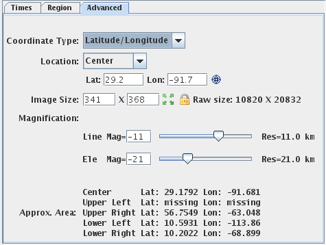
The image properties in the Advanced tab allow you to override the default properties McIDAS-V uses to specify aspects of the image data. The widgets show the defaults McIDAS-V will use. By changing any of the widgets you can override the default value.
Use the Stride tab to change the number of points used to create the image. You can utilize fewer points along the X and Y-axes to display the data faster, but with less precision. It is recommended to leave the X and Y values as their default (All points) unless you are trying to get a general picture and nothing too specific.
Use the Settings tab to utilize any display settings you may have set.
The Subsetting component of the Field Selector allows you to subset the data in both time and space (if possible). If there are times in the data source you are viewing they will be shown in this area. Likewise, if it is possible to do spatial subsetting or decimation a Spatial Subset tab will be shown.
Time and spatial subsetting defaults can be applied to the data source itself through the Data Source Properties dialog or the defaults can be overwritten through the Field Selector tab.
The Layer Controls tab of the Data Explorer is used to modify an existing display. The options to choose from in this tab will vary depending on your data source and field selected.
This section describes the specifics of the Layer Controls tab for different data sources and fields, including the following:
There are some general features of the Layer Controls tab that are consistent with every display, which are described below.
![]() - Provides a dropdown menu with options to move the Main Display window to the front displaying the selected tab, and allows you to access the View and Projections menus of the Main Display window.
- Provides a dropdown menu with options to move the Main Display window to the front displaying the selected tab, and allows you to access the View and Projections menus of the Main Display window.
These options are found at the bottom left corner of the Layer Controls tab of the Data Explorer.

All parameters share a common set of File, Edit, View, and Help menu items, shown in the menu bar of the Layer Controls tab. Different controls may also have custom items in these menus as well.
The File menu has these common choices:
The Edit menu has these common choices:
The View menu has these common choices:
Plan views can be made in four types of displays: Contour Plan View, Color-Filled Contour Plan View, Color-Shaded Plan View, and Value Plots. Contour Plan View and Color-Filled Contour Plan View have the same properties. For more information on the Value Plots display, see Value Plot Controls.
Many of the menu items seen utilizing this display are standard options that can be found in the Menus section of the Layer Controls page. However, there are some options that are unique to this display.
The Edit menu has these unique options:
The View menu has this unique option:
The Flow Plan View Controls are used to control plan (horizontal) displays (flow vectors, wind barbs, streamlines) of vector based data (e.g., wind components). They are similar to the Plan View controls. For more information on what wind speeds correspond to each of the wind barbs in McIDAS-V displays, please see the table in the FAQ.
The five types of Flow Displays are Vector Plan View, Streamline Plan View, Wind Barb Plan View, Vector Cross Section, and Wind Barb Cross Section. When you are working with 3D data, you can select Vectors Over Topography, Wind Barbs Over Topography, and Streamlines Over Topography. The Layer Controls listed below apply for all display types:
 or
put in a value and hit enter to change the value.
or
put in a value and hit enter to change the value.Many of the menu items seen utilizing this display are standard options that can be found in the Menus section of the Layer Controls page. However, there are some options that are unique to this display.
The Edit menu has these unique options:
The View menu has this unique option:
The Value Plot controls are used to adjust the display of individual grid point values.
Many of the menu items seen utilizing this display are standard options that can be found in the Menus section of the Layer Controls page. However, there are some options that are unique to this display.
The Edit menu has these unique options:
The View menu has this unique option:
The Vertical Cross Section Controls are used to adjust vertical cross section displays. Vertical cross sections can be made in three types of displays: Contour, Color-Filled Contour, and Color-Shaded. The control window has two tabs: Display and Settings. You can change the endpoints of the cross section by clicking and dragging the endpoints in the Main Display window.
The Display tab includes a duplicate of the display in the Main Display window:
The Settings tab shows the settings for this display control:
Many of the menu items seen utilizing this display are standard options that can be found in the Menus section of the Layer Controls page. However, there are some options that are unique to this display.
The Edit menu has this unique option:
The View menu has these unique options:
Isosurfaces can be made in two types of displays, regular isosurfaces, and isosurfaces colored by another parameter. An isosurface is a 3D surface mapping the location of a single parameter value through a 3D field. Isosurfaces are a 3D analog of a single contour line in a 2D plot; the intersection of an isosurface and any plane is a contour line of the same value in that plane.
Coloring an isosurface by another parameter can serve many purposes. One example use of this is creating a display for possible icing conditions in the atmosphere that could be useful for pilots. To do this, you would select Temperature as your field, the "Isosurface colored by another parameter" display type, and Relative Humidity in the Field Selector window that appears when you click Create Display. After the display is created, you can set the isosurface value for Temperature to be 0 degrees Celsius in the Layer Controls tab of the Data Explorer. Now, in the Main Display window, you have a surface of 0 degrees Celsius colored by Relative Humidity. Wherever you see high RH values means that there is a lot of moisture in the atmosphere, and at the freezing temperatures, there could be icing conditions.
 button or entering a
value in the field and hitting Enter.
button or entering a
value in the field and hitting Enter.Many of the menu items seen utilizing this display are standard options that can be found in the Menus section of the Layer Controls page. However, there is one option that is unique to this display.
The Edit menu has this unique option:
The View menu has this unique option:
3D grids can be rendered as a volume display.

You can use the transparency features of the color table to see through the display. This is done by right-clicking on the color bar, going down to Transparency, and selecting a percentage.
Many of the menu items seen utilizing this display are standard options that can be found in the Menus section of the Layer Controls page. However, there is one option that is unique to this display.
The View menu has this unique option:
The Point Volume display shows the grid points in a volume of data as individual points in the display. The controls are used to change color tables, the number of points to skip, and the point size.
You can use the transparency features of the color table to see through the display. This is done by right-clicking on the color bar, going down to Transparency, and selecting a percentage.
Many of the menu items seen utilizing this display are standard options that can be found in the Menus section of the Layer Controls page. However, there is one option that is unique to this display.
The View menu has this unique option:
For 3D derived gridded data, one of the Fields you can select is Sounding Data (Temperature & dewpoint only or with true winds). In the Displays panel of the Layer Controls tab, there is a category for soundings. The three sounding display options are Grid Skew-T, Grid Stuve Display, and Grid Emagram Display. This display uses the model data to produce soundings, and their controls are similar to those for Point Data sounding display controls. You can modify the location of the sounding in the Main Display window by dragging the selector point to a different position on the map.
The example below is loaded from the 'Sounding Data (with true winds)' field. If you select 'Sounding Data (Temperature & dewpoint only)', then wind data will not be included in the display. Therefore, there will be no barbs along the side of the sounding in the Sounding Chart tab, the Hodograph tab will not be available, and there will be no wind information listed in the Table tab. For more information on what wind speeds correspond to each of the wind barbs in McIDAS-V displays, please see the table in the FAQ.
The Sounding Chart tab includes an aerological diagram (e.g., skew-T, Stuve, Emagram):
A label above the sounding's chart shows the model, date, and time of the data. You can modify the individual T and Td profiles on the skew T by clicking and dragging the profile lines. You will see changes in the parameter table to the left of the Skew-T that reflect modifications made to the sounding.
The Hodograph tab shows a 3D hodograph display. Note that this tab is only included with the display if you select a Field that includes wind data:
The hodograph is enabled if the plotted data includes wind fields. It can be rotated into 3D by right-clicking and dragging. You can zoom in/out by holding down Shift and right-clicking and dragging up/down or by using the scroll wheel on your mouse. To reset the hodograph, use Ctrl+R.
The Table tab shows a table of all available values in the sounding. You can invert the order of the table by double clicking on the name of a column (ex. AirPressure).:
The table to the left of the sounding diagram contains aerological parameters determined from the atmospheric sounding displayed in the diagram. The following abbreviations are used:
Many of the menu items seen utilizing this display are standard options that can be found in the Menus section of the Layer Controls page. However, there is one option that is unique to this display.
The File menu has this unique option:
The Edit menu has these unique options:
The View menu has these unique options:
The Hovmoller display plots grid and gridded point data in a diagram with the Latitude/Longitude component on the X-axis, and the time component on the Y-axis. This display option is found in the Displays menu of the Field Selector tab of the Data Explorer. You can display the data as Time with respect to either Latitude or Longitude, and either as a Color Shaded or Contour display type.
By default, if you select a Longitude display, the entire spatial domain will be utilized, and the longitude range will go from the western extent to the eastern extent of your domain. The latitude will be averaged from the northern to southern boundaries of your domain. You can restrict the latitude and longitude domain by selecting a region in the Region tab of the Field Selector tab of the Data Explorer. The Latitude displays work the same way, by averaging the longitude across the entire domain unless you subset a region.
Many of the menu items seen utilizing this display are standard options that can be found in the Menus section of the Layer Controls page. However, there are a couple of options unique to this display.
The Edit menu has this unique option:
The View menu has this unique option:
The Trajectory Colored By Parameter display type is capable of working with gridded data containing u and v-wind components, as well as a scalar quantity to color them by. You can create both 2D and 3D trajectories dependent on what is contained in your data. To use this display type, you can use the grid formulas Grid 2D Trajectory or Grid 3D Trajectory. These formulas will request for your scalar quantity, as well as individual u and v-wind fields. An alternative to the formulas is utilizing the new derived 2D and 3D fields of your data, Grid 2D Trajectory and Grid 3D Trajectory. When using these fields, all you need to specify is the scalar quantity, and McIDAS-V will pull out the relevant u and v-wind components (as well as the vertical component when creating 3D Trajectories).
After clicking Create Display and choosing your field(s), you will arrive at the Layer Controls tab of the Data Explorer, where you will define the properties of your trajectories.
Once you click ![]() to create your trajectories, the options in the Layer Controls will expand to include more controls. This is composed of two tabs: Layout, and Times.
to create your trajectories, the options in the Layer Controls will expand to include more controls. This is composed of two tabs: Layout, and Times.
The Layout tab allows you to set various aesthetic aspects of your display:
The Times tab allows you to determine how many times are included with each trajectory.
This time setting is different than that used for the general Define Animation Times tab of the Time Animation Widget since it has no influence on the number of time steps in the loop, but rather the amount of data shown at each time step. You can utilize various options for Start Time and End Time to determine how much of each trajectory will be shown at each time step.
Many of the menu items seen utilizing this display are standard options that can be found in the Menus section of the Layer Controls page. However, there are a couple of options unique to this display.
The File menu has these unique options:
The Image Controls are used to adjust displays of satellite imagery. The control window generally consists of two tabs: Settings and Histogram.
The Settings tab allows you to customize many aspects of the appearance of your display. Note that the items in this control may be different depending on which display type you select:
The Histogram tab allows you to visualize a histogram of your Satellite data:
There are many ways that you can customize this histogram. If you right-click on the histogram and select Properties, you can get to a Plot Properties dialog which allows you to change many aesthetic properties of the histogram. You can also modify the display in the Main Display window through the Histogram tab. You can do this by left-clicking and dragging from left to right to zoom in over your desired range of data values. Once you are done zooming in, the display in the Main Display window will modify to use a color bar range that matches the boundaries of the zoom box you created in this tab. To return to the original data range, use the ![]() button.
button.
One of the display types in the Displays subset panel of the Field Selector is Image Display Over Topography. This display type differs from the other Imagery display types because it allows you to create a 3D display of your satellite image. In order to utilize this display type, you must have both the satellite data and a separate data source for topography. One example of a topographic data source is the 2D->Geopotential_height @ surface field of GFS CONUS model data.
To use this display type, select your satellite field, the Image Display Over Topography display type, and click Create Display. This will open a Field Selector window, prompting for your topography field. Once you select your topography field and click OK, a 3D display of your satellite image draped over topography will be displayed. You can rotate the image in the Main Display window using right-click and drag to visualize the 3D aspects of the display. You can also make the topographic features stand out more or less by using the Vertical Range item in the Viewpoint Toolbar in the Main Display window. Lowering the Max value field of the Vertical Range window will make tall features (ex. mountains) appear even taller.
The Layer Controls tab of the Data Explorer for this display type does not include a Histogram tab. The controls in this tab are Color Table, Pixel Sampling, and Texture Quality, which are described in the Properties section above.
Note: In order to get this display type to show 3D topographic features, the entire domain of your satellite data must lie within the domain of your topographic field. For example, if you are working with a full disk satellite image, but you only have topographic data over the United States, you must subset a satellite region over the United States in the Region tab of the Field Selector before creating the display. If you do not do this, the image will display entirely in the 2D and not show any topographic features.
Many of the menu items seen utilizing this display are standard options that can be found in the Menus section of the Layer Controls page. However, there is one option that is unique to this display.
The View menu has this unique option:
HYDRA MultiSpectral Display controls are used to create a multispectral display within McIDAS-V. There are two sets of controls, the MultiSpectral Display and the MultiSpectral Probes. The Multispectral Display consists of three tabs: Display, Settings, and Histogram.
The Display tab shows the spectra. This may differ if you are looking at Hyperspectral data or Multispectral data due to the number of bands included with the data. Hyperspectral data will have a spectra drawn as a line, while multispectral data will show a variety of points:
Use the Shift+left click+drag combination to create a box of a region to zoom in on. To return to the full spectra, use Ctrl+left click. Middle-clicking on a point in the spectra will change the wavelength/wavenumber of the image displayed. Right click+drag will translate the spectra left or right. Left click+drag on the green wavelength/wavenumber selector bar will allow you to change the wavelength displayed in the image. As you are dragging the selector bar, the wavelength/wavenumber will be displayed in the upper left corner of the spectra window for the current location of the the bar.
The Settings tab shows the settings for this display control and the readout probes:
The Histogram tab shows the histogram of the data for the image:
Zoom in by left-clicking and dragging on the histogram, or enter in a set of minimum and maximum values.
Many of the menu items seen utilizing this display are standard options that can be found in the Menus section of the Layer Controls page. However, there is one option that is unique to this display.
The View menu has this unique option:
The Linear Combinations controls are used to create and perform functions beyond the standard arithmetic functions in McIDAS-V. The Console tab consists of two parts - The Spectra and the Console:
The Console allows a user to define multiple spectra and perform more complex mathematical operations.
| a = selector() | [ Creates a green selector named "a" at a data-dependent wavenumber or wavelength] |
| b = selector(1000) | [ Creates a green selector named "b" at wavenumber 1000.0 ] |
| c = selector('cyan') | [ Creates a cyan selector named "c" at a data-dependent wavenumber or wavelength] |
| d = selector(919.5, 'red') | [ Creates a red selector named "d" at wavenumber 919.5 ] |
| e = selector('40', 'orange') | [ Creates a orange selector named "e" at the wavenumber? associated with band 40 ] |
| f = selector('11') | [ Creates a green selector named "f" at the wavenumber associated with band 11 ] |
| a = selector('2', 'red') | [ Creates a red selector named "a" at the wavenumber associated with band 2] |
| b = selector('1', 'yellow') | [ Creates a yellow selector named "b" at the wavenumber associated with band 1] |
| c = ((a-b)/(a+b)) | [ Creates a variable c that corresponds to the expression ((a-b)/(a+b))] |
| combine(c, 'NDVI') | [ Results of the "c" variable will appear in the Field Selector as the "NDVI" entry ] |
| combine((a-b)/(a+b)) | [ Results of the expression in the combination field will appear in the Field Selector ] |
The 4 Channel Combination controls are used to create a basic linear combination of spectral bands. There are two sets of controls. The top of the controls shows the spectra, while the bottom half gives the linear combination option:
Use the Shift+left click+drag combination to create a box of a region to zoom in on. To return to the full spectra, use Ctrl+left click. The Middle click+drag probing feature will list the wavelength/wavenumber as well as the reflectance or Brightness Temperature at a point along the spectra. Use the Left click+drag option to move the spectra selector bar(s) to a different value. The new value for where you moved the spectra bar to will be updated in the field at the bottom of the window.
The 4 Channel Combination tool allows you to specify arithmetic expressions for four spectral bands. Use the pull down menus between variables to select the appropriate arithmetic expressions for the equation. To apply a multiplier to any of the variables, change the value ahead of the wavelength/band.
The controls for Level III Radar imagery are similar to the standard Image Controls and are used to adjust image displays of this Radar imagery. The control window consists of two tabs: Settings and Histogram.
The Settings tab allows you to customize many aspects of the appearance of your display:
The Histogram tab allows you to visualize a histogram of your Radar data:
There are many ways that you can customize this histogram. If you right-click on the histogram and select Properties, you can get to a Plot Properties dialog which allows you to change many aesthetic properties of the histogram. You can also modify the display in the Main Display window through the Histogram tab. You can do this by left-clicking and dragging from left to right to zoom in over your desired range of data values. Once you are done zooming in, the display in the Main Display window will modify to use a color bar range that matches the boundaries of the zoom box you created in this tab. To return to the original data range, use the ![]() button.
button.
Many of the menu items seen utilizing this display are standard options that can be found in the Menus section of the Layer Controls page. However, there is one option that is unique to this display.
The View menu has this unique option:
The Radar Sweep Controls are used to control displays of single level sweeps of radar data, and their display appears in the Main Display window. WSR-88D Level II radar data has three moments or display types: Reflectivity, RadialVelocity, and SpectrumWidth, indicated by the ![]() icon in the Field Selector. WSR-88D Dual Pole radar includes these three moments, as well as DifferentialReflectivity, CorrelationCoefficient, and DifferentialPhase.
icon in the Field Selector. WSR-88D Dual Pole radar includes these three moments, as well as DifferentialReflectivity, CorrelationCoefficient, and DifferentialPhase.
The controls are identical for 2D and 3D displays:
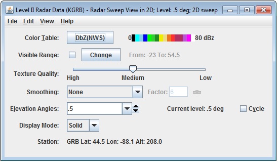
Many of the menu items seen utilizing this display are standard options that can be found in the Menus section of the Layer Controls page. However, there are some options that are unique to this display.
The Edit menu has this unique option:
The View menu has this unique option:
The RHI (Range-Height Indicator) display appears in the Main Display window and as a 2D plot in the Layer Controls tab. WSR-88D Level II Radar data has three moments or data types: Reflectivity, Radial Velocity, and Spectrum Width, indicated by the ![]() icon in the Field Selector. WSR-88D Dual Pole radar includes these three moments, as well as DifferentialReflectivity, CorrelationCoefficient, and Differential Phase. In order for RHI to be listed as a valid Display Type in the Field Selector, one of the moments (ex. Reflectivity, RadialVelocity, etc.) must be chosen in the Fields panel, not one of their individual elevation angles. The control window contains
two tabs, Display and Settings.
icon in the Field Selector. WSR-88D Dual Pole radar includes these three moments, as well as DifferentialReflectivity, CorrelationCoefficient, and Differential Phase. In order for RHI to be listed as a valid Display Type in the Field Selector, one of the moments (ex. Reflectivity, RadialVelocity, etc.) must be chosen in the Fields panel, not one of their individual elevation angles. The control window contains
two tabs, Display and Settings.
The Display tab shows the RHI in 2D:
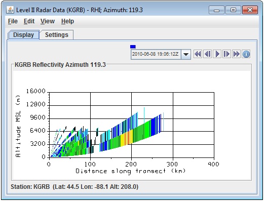
The Settings tab shows settings to control the display:
Many of the menu items seen utilizing this display are standard options that can be found in the Menus section of the Layer Controls page. However, there are a couple of options that are unique to this display.
The View menu has this unique option:
The Edit menu has this unique option:
The radar vertical Cross Section Control is used to adjust vertical cross section displays of Level II Radar volume data. WSR-88D Level II Radar data has three moments or data types: Reflectivity, Radial Velocity, and Spectrum Width, indicated by the ![]() icon in the Field Selector. WSR-88D Dual Pole radar includes these three moments, as well as DifferentialReflectivity, CorrelationCoefficient, and Differential Phase. In order for Radar Cross Section to be listed as a valid Display Type in the Field Selector, one of the moments (ex. Reflectivity, RadialVelocity, etc.) must be chosen in the Fields panel, not one of their individual elevation angles. The control window has two tabs, Display and Settings.
icon in the Field Selector. WSR-88D Dual Pole radar includes these three moments, as well as DifferentialReflectivity, CorrelationCoefficient, and Differential Phase. In order for Radar Cross Section to be listed as a valid Display Type in the Field Selector, one of the moments (ex. Reflectivity, RadialVelocity, etc.) must be chosen in the Fields panel, not one of their individual elevation angles. The control window has two tabs, Display and Settings.
The Display tab includes a duplicate of the display in the Main Display window:
The Settings tab shows the settings for this Layer Control:
Many of the menu items seen utilizing this display are standard options that can be found in the Menus section of the Layer Controls page. However, there is one option that is unique to this display.
The View menu has this unique option:
The CAPPI (Constant Altitude Plan Position Indicator) Radar display appears in the Main Display window. WSR-88D Level II Radar data has three moments or data types: Reflectivity, Radial Velocity, and Spectrum Width, indicated by the ![]() icon in the Field Selector. WSR-88D Dual Pole radar includes these three moments, as well as DifferentialReflectivity, CorrelationCoefficient, and Differential Phase. In order for CAPPI to be listed as a valid Display Type in the Field Selector, one of the moments (ex. Reflectivity, RadialVelocity, etc.) must be chosen in the Fields panel, not one of their individual elevation angles.
icon in the Field Selector. WSR-88D Dual Pole radar includes these three moments, as well as DifferentialReflectivity, CorrelationCoefficient, and Differential Phase. In order for CAPPI to be listed as a valid Display Type in the Field Selector, one of the moments (ex. Reflectivity, RadialVelocity, etc.) must be chosen in the Fields panel, not one of their individual elevation angles.
The CAPPI Radar displays data at a constant altitude around the Radar site:
The Layer Controls tab of the Data Explorer allows for several ways to customize the image or loop displayed:
Many of the menu items seen utilizing this display are standard options that can be found in the Menus section of the Layer Controls page. However, there is one option that is unique to this display.
The View menu has this unique option:
The radar volume scan controls are used to show a radar volume as a series of nested cones. WSR-88D Level II Radar data has three moments or data types: Reflectivity, Radial Velocity, and Spectrum Width, indicated by the ![]() icon in the Field Selector. WSR-88D Dual Pole radar includes these three moments, as well as DifferentialReflectivity, CorrelationCoefficient, and Differential Phase. In order for Radar Cross Section to be listed as a valid Display Type in the Field Selector, one of the moments (ex. Reflectivity, RadialVelocity, etc.) must be chosen in the Fields panel, not one of their individual elevation angles.
icon in the Field Selector. WSR-88D Dual Pole radar includes these three moments, as well as DifferentialReflectivity, CorrelationCoefficient, and Differential Phase. In order for Radar Cross Section to be listed as a valid Display Type in the Field Selector, one of the moments (ex. Reflectivity, RadialVelocity, etc.) must be chosen in the Fields panel, not one of their individual elevation angles.
Many of the menu items seen utilizing this display are standard options that can be found in the Menus section of the Layer Controls page. However, there is one option that is unique to this display.
The View menu has this unique option:
Displays of Level II isosurfaces are controlled by the Isosurface controls. The Radar Isosurface display type allows you to visualize radar data in the 3D, including all elevation angles, at specific data values. An example of when this display type can be useful is if you are looking for only very high reflectivity values that may coincide with a hail spike. WSR-88D Level II Radar data has three moments or data types: Reflectivity, Radial Velocity, and Spectrum Width, indicated by the ![]() icon in the Field Selector. WSR-88D Dual Pole radar includes these three moments, as well as DifferentialReflectivity, CorrelationCoefficient, and Differential Phase. In order for Radar Isosurface to be listed as a valid Display Type in the Field Selector, one of the moments (ex. Reflectivity, RadialVelocity, etc.) must be chosen in the Fields panel, not one of their individual elevation angles.
icon in the Field Selector. WSR-88D Dual Pole radar includes these three moments, as well as DifferentialReflectivity, CorrelationCoefficient, and Differential Phase. In order for Radar Isosurface to be listed as a valid Display Type in the Field Selector, one of the moments (ex. Reflectivity, RadialVelocity, etc.) must be chosen in the Fields panel, not one of their individual elevation angles.
 button or by entering a value in the text field and pressing Enter.
Many of the menu items seen utilizing this display are standard options that can be found in the Menus section of the Layer Controls page. However, there is one option that is unique to this display.
The View menu has this unique option:
The Profiler Time/Height display shows winds at all levels above one station, for one or more times. Winds are shown with the meteorological wind barb symbol. The location of the barb on the plot shows the wind observation height above mean sea level, and the barb provides information about the direction and speed of the wind. For more information on what wind speeds correspond to each of the wind barbs in McIDAS-V displays, please see the table in the FAQ.
The map position of the vertical profile is indicated by the "Lat: Long:" readout above the graph. The time and height values on the plot can be sampled by dragging the middle mouse button over the plot.
Many of the menu items seen utilizing this display are standard options that can be found in the Menus section of the Layer Controls page. However, there is one option that is unique to this display.
The View menu has this unique option:
The Profiler Station Plot display shows winds at one level above one or more stations on the Main Display window. Winds are shown with the wind barb symbol. For more information on what wind speeds correspond to each of the wind barbs in McIDAS-V displays, please see the table in the FAQ.
All of the menu items seen utilizing this display are standard options that can be found in the Menus section of the Layer Controls page.
The Profiler 3D View shows winds at all levels above one or more stations in the Main Display window. Winds are shown with the wind barb symbol. For more information on what wind speeds correspond to each of the wind barbs in McIDAS-V displays, please see the table in the FAQ.
All of the menu items seen utilizing this display are standard options that can be found in the Menus section of the Layer Controls page.
The Data Probe/Time Series display shows a time series chart of one or more fields at a single location. It also shows a tabular readout of the value at the current animation time step. Note that you must select two or more times in the Field Selector in order to get valid data to display in the charts. In the image below we have a Probe Control showing three parameters: T, RH and windspeed. Their values at the current animation time step are shown in the table and their time series are shown. Note, the T and RH fields are shown in one chart and the windspeed is shown in another chart. You can have any number of fields and any number of charts. You can configure the layout of the charts, the chart properties and the line properties for each parameter. See the Charts page for more information.
A small colored square selector point in the Main Display window shows the location of the data probe. You can drag the data probe over the map in the Main Display window by using left-click and drag. When displaying a 3D field, you can change the data probe vertically as well. As the selector point is moved, the data in the charts will change to represent the data at the location of the probe.
The table shows the parameters with their values, the level at which the value is sampled, and the type of sampling. At the bottom of the window, the location of the probe is shown in latitude, longitude, and altitude. When surface data is probed the height of the probe point does not matter. You can move the probe by clicking and dragging it in the Main Display window, or by entering new values into the Lat, Lon, and Alt fields and pressing Enter.
You can add new parameters a number of ways:
These parameter actions can be accessed by right-clicking on the parameter row in the table or through the View->Parameters menu.
When probing on point data, the control will find the closest observation to the probe position and use that data to sample on.
Many of the menu items seen utilizing this display are standard options that can be found in the Menus section of the Layer Controls page. However, there are several menu options that are unique to the Data Probe/Time Series display. These menus are found at the top of the Layer Controls tab of the Data Explorer.
The File Menu has these unique options -
The Edit Menu has these unique options -
The View Menu has these unique options -
A Time/Height Display is a display of samples of a 3D parameter along a vertical profile line from top to bottom of the available data, with time as the independent coordinate (X-axis). You can choose both a Contour or Color Shaded Time/Height Display.
Many of the menu items seen utilizing this display are standard options that can be found in the Menus section of the Layer Controls page. However, there are some options that are unique to this display.
The Edit menu has these unique options:
The View menu has these unique options:
The Vertical Profile Display Control shows a plot of any number of field values versus altitude. See the Charts page for more information about customizing the chart. In order to use the Vertical Profile display, you must be working with 3D data.
The map position of the profile is shown in the Main Display window by a colored vertical line. There is a Selector Point on top of the vertical line. You can move the vertical profile line by dragging the Selector Point with the left mouse button.
Many of the menu items seen utilizing this display are standard options that can be found in the Menus section of the Layer Controls page. However, there are some options that are unique to this display.
The Edit menu has these unique options:
The View menu has these unique options:
The Data Transect controls are used to adjust data transect displays. The control window includes a display of the profile of the data along the transect. The vertical axis is the parameter value and the horizontal axis is the distance along the transect line. In the Main Display window, a transect selector allows you to position the location of the transect by dragging the selector points along the line. The control window consists of two tabs, Display and Settings.
The Display tab shows the the profile of the data along the transect:
The Settings tab contains widgets for changing properties of that display:
Many of the menu items seen utilizing this display are standard options that can be found in the Menus section of the Layer Controls page. However, there are several options that are unique to this display.
The Edit menu has these unique options:
The View menu has these unique options:
Maps in McIDAS-V are shown using the Map Display Controls. There are two ways these controls are used: for the default background maps and for a user created map display. The control window is composed of two tabs, Maps and Lat/Lon.
The Maps tab lists the set of available maps. You have the ability to select which maps are displayed, as well as how they are displayed:
The Lat/Lon tab allows the user to set the visibility of and control the latitude/longitude lines and labels:
Many of the menu items seen utilizing this display are standard options that can be found in the Menus section of the Layer Controls page. However, there are some options that are unique to this display.
The File menu has this unique option:
The Edit menu has these unique options:
The View menu has this unique option:
The Topography controls allow you to display topography datasets. These controls are available through the 3D Surface->Topography display type. An example of a field that can utilize this display type is the 2D 'Geopotential Height @ Surface' field in model data. The first image shows the control user interface which allows you to customize many options with this display.
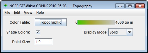
This is an example of how the display may appear in the Main Display window:
Many of the menu items seen utilizing this display are standard options that can be found in the Menus section of the Layer Controls page. However, there is one option that is unique to this display.
The View menu has this unique option:
McIDAS-V supports the ability to load and display GIS shapefiles. You can select and load a shape file (i.e., a file that ends with .shp) from the General->Files/Directories chooser in the Data Sources tab of the Data Explorer using the Shapefile Data Type. The zipped (.zip) version of shapefiles can also be loaded.
For shapefiles that also have a data base file (.dbf) you can control what shape segments are shown with the Filters tab.
Note: McIDAS-V supports a simple XML format for maps. The Shapefile Control can export the displayed shapes in this XML format the File->Save->Export Displayed Shapes... menu.
When the shapefile has an associated data base file (.dbf) a tabular listing of the attributes is shown in the Table tab. Use the Select Fields to Show button to select what fields to show. The table can be exported as a CSV file with the File->Save->Export Table... menu.
Many of the menu items seen utilizing this display are standard options that can be found in the Menus section of the Layer Controls page. However, there is one option that is unique to this display.
The Edit menu has this unique option:
The Point Data Plot Control displays a set of observations using a station model. This control is accessed by selecting the Point Data field and the Point Data Plot display. The control window consists of four tabs: Layout, Times, Plot, and Filters.
The Layout tab allows you to control basics of the display:
The Times tab allows you to change the observation times that are shown in the display. By default, data for a single time corresponding to the current animation time will be shown. Using this widget allows you to show data from multiple times at once:
Clicking ![]() opens a Time Settings window that allows you to select specific start and end times:
opens a Time Settings window that allows you to select specific start and end times:
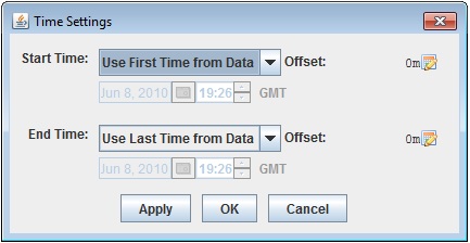
Image 3: Time Settings Dialog
The Plot tab provides a time series chart and a data readout table of a selected station. To use this, left-click on a station in the main display. Double-click or right-click and select Add To Chart on a table row to add it to the time series chart. See the Charts page for more information about customizing the chart:
The Filters tab allows you to set individual or multiple filters to specify which data are shown in the Main Display window:
As an example, the above image shows two filter expressions, one that states the Temperature Property needs to be greater that 35 F and the other states that the Wind Speed value needs to be greater than 15. The unit of [F] is entered for the Temperature Property. If you do not define a unit after the value, then McIDAS-V will utilize the native unit for the Property. Match all of the filters is selected, meaning only station models where the Temperature is greater than 35 degrees F and the wind speed is greater than 15 will be plotted in the Main Display window.
Many of the menu items seen utilizing this display are standard options that can be found in the Menus section of the Layer Controls page. However, there are some options that are unique to this display.
The File menu has these unique options:
The Edit menu has this unique option:
The View menu has these unique options:
The Point Data List Control shows a set of observation data in a textual list format. This control is accessed by selecting the Point Data field and the Point Data List display.
The ![]() button opens a Field Selector window that allows you to determine which fields are included in the table:
button opens a Field Selector window that allows you to determine which fields are included in the table:
Many of the menu items seen utilizing this display are standard options that can be found in the Menus section of the Layer Controls page. However, there is one option that is unique to this display.
The File menu has this unique option:
McIDAS-V can create gridded fields of numeric data using the Barnes Objective Analysis. You can control the parameters used to create the grid from the Data Source Properties or using the Grid Parameters tab in the Data Subset panel of the Field Selector. Note that since this gridded display will utilize point observation data, the display over areas with few observations (ex. open ocean) may not correctly represent the actual data over that region. To get more exact gridded displays of point data, it is best to utilize the Region tab to subset an area of interest with a relatively high density of point observations:
The resulting grid can be displayed using any of the Gridded Data Displays.
The meteorological sounding display is available for: RAOBs, numerical weather prediction model output, and from a local file that contains aircraft track data. The dewpoint temperature is computed by internal code from temperature and relative humidity grids.
To load sounding data see Choosing RAOB Sounding Data and Displaying Gridded Data. The sounding display consists of a table of aerological (thermodynamic) parameters and three tabs: Sounding Chart, Hodograph, and Table.
The Sounding Chart tab includes an aerological diagram (e.g., skew-T, Stuve, Emagram):
A label above the sounding's chart shows the station number, date, and time of the sounding. When displaying sounding plots made from gridded model output, the position of the sounding is shown in the Main Display window by a solid-color selector point and vertical line. You can move this model-output-based sounding position over the map by dragging the selector point with the left mouse button.
When displaying a sounding diagram made from gridded numerical weather model output, there is a pull-down selector menu of the model output valid times in the upper right corner.
The animation control buttons are available in either case:
To increase precision using the sounding diagram, enlarge the window by dragging on the edges. You can zoom the sounding diagram by holding down the Shift key and dragging the right button upwards; drag downwards to zoom out. Zooming can also be done by using the scroll wheel on the mouse. You can pan the diagram by dragging the mouse pointer in any direction while holding down the right mouse button.
The temperature and dewpoint traces can be modified via the cursor. Press the left button on the first data-point to be modified and drag it horizontally along an isobar to the desired position, then move the pointer diagonally along an isotherm to keep the data-point at the desired position and to pick-up the next data-point. Repeat until done and then release the mouse button.
The Hodograph tab shows a 3D hodograph display:
The hodograph is enabled if the plotted data includes wind fields. It can be rotated into 3D by clicking and dragging the right mouse button. You can zoom in/out by holding down Shift and right-clicking and dragging up/down or by using the scroll wheel on the mouse. To reset the hodograph, use Ctrl+R.
The Table tab shows a table of all values in the sounding:
The table to the left of the sounding diagram contains aerological parameters determined from the atmospheric sounding displayed in the diagram. The following abbreviations are used:
Many of the menu items seen utilizing this display are standard options that can be found in the Menus section of the Layer Controls page. However, there are some options that are unique to this display.
The File menu has this unique option:
The Edit menu has these unique options:
The View menu has these unique options:
The Front Controls shows a list of the different weather features (high and low pressures, fronts, etc.) shown in the Main Display window in a textual list format. This control becomes available once the Front Positions data source has been added:
Double-clicking on an item in this window open the Properties Editor for that item. This window consists of two tabs: Properties and Points:
The Properties tab allows you to change general characteristics of the display. Note that the options that appear in this tab may differ depending on what feature's properties you are viewing:
The Points tab provides information about the location of the selected feature:
All of the menu items seen utilizing this display are standard options that can be found in the Menus section of the Layer Controls page.
McIDAS-V provides a collection of locations. These may be NEXRAD stations, states, counties, geographical features, countries, etc. The Location Controls are used to display these locations. The list of locations is accessed through the Display->Plot Location Labels... menu item in the Main Display window. You can also load in local files that use these location controls. The user interface consists of four tabs: Display, Locations, Data Sets, and Filters.
The Display tab allows the user to control how the display will appear in the Main Display window:
The Locations tab shows two sub-tabs, All Locations and Displayed Locations. Shown at the bottom are the details of a location:
The Data Sets tab lists all of the location files that are being displayed. You can remove a data set by clicking on the data set and pressing Delete:
The Filters tab allows you to filter what locations are being shown based on their internal attributes:
Many of the menu items seen utilizing this display are standard options that can be found in the Menus section of the Layer Controls page. However, there are some options that are unique to this display.
The Edit menu has these unique options:
The View menu has these unique options:
The WorldWind controls are a special version of the Location Controls. They provide access to a large collection of locations from NASA's WorldWind Viewer project.
As the display is panned or zoomed over more locations, different location sets are retrieved and displayed.
The track controls display trajectory data sets, e.g., aircraft track, ship, buoys, etc. This data can be loaded in the General->Files/Directories chooser of the Data Sources tab of the Data Explorer, with the Data Type of Track files. You can display your data in the form of a chart, table, track, or as a Point Data Plot drawn in the Main Display window. The items in the Layer Controls for a Point Data plot are the same as the controls for displaying regular Point Data. If you are working with data for a lot of times, or have many parameters included with your data, you may be prompted to subset the point data. This gives you the option of only including the necessary fields to cut down on memory usage and time to display the data.
To draw a track in the Main Display window, select your field in the Fields panel, the Track Colored By Parameter display type, and hit Create Display. These same controls are utilized for the Trajectory Colored By Parameter display type. The track controls consist of two tabs, Layout and Times.
The Layout tab controls the appearance of the display:
The second tab controls the Times used for the display:
This dialog allows you to define the time range to show of the track. The image above defines that the end time is the current animation time, and the start time is relative to the end time less 30 minutes. This means that the track or trajectory drawn in the Main Display window would include the current animation time of the loop, as well as the any data from 30 minutes prior this time.
This time setting is different that that used for the Define Animation Times tab of the Time Animation Widget since it has no influence on the number of time steps in the loop, but rather the amount of data shown at each time step. You can utilize the various options for Start Time and End Time to determine how much of the track or trajectory will be shown in each time step.
Many of the menu items seen utilizing this display are standard options that can be found in the Menus section of the Layer Controls page. However, there is one item that is unique to this display.
The Edit menu has this unique option:
The View menu has this unique option:
The Scatter Analysis controls are used to create a scatter plot within McIDAS-V. The scatter controls show three different panels:
The plot on the first panel on the left represents the first field selected in the Field Selector, the panel in the middle represents the second field which is selected through the Field Selector window, and the panel on the right is the scatter analysis of the two fields. The first field selected is represented on the X-axis (abscissa) and the second field selected represents the Y-axis (ordinate). The X-axis is selected in the Field Selector - what you have selected in the lower right Channels tab will be used as the X-axis.
You can subset regions in any of the three panels, and the equivalent points will also be selected in the other two panels. For example, if you draw a box in panel 1, the same box will be drawn in panel 2, and the points in these boxes will be colored the same in panel 3, the scatter analysis. To draw a box, select a Box radio icon and a color, and use Shift+left-click and drag to select a region. You can also draw any enclosed shape by selecting the Curve radio button and a color, and left-click and drag in any panel to select a region. You are allowed one box and one curve per color in the scatter analysis (panel 3), and one box and one curve for the images (panels 1 and 2). To remove region that you have subsetted, simply double click on the color of the region you wish to remove next to the Box/Curve radio buttons.
Right-click on the color bar below the images to open the Color Table Editor, change the range, select other color tables, etc.
To the right of the Box/Curve options, there is a ![]() button. Clicking this button will Scatter Statistics window that will list statistical information about the data as a whole, as well as the regions of the data that were subsetted with a box/curve. The values in the white columns are computed for the image as a whole, and the values in the colored columns are computed for the area of the respective box/curve.
button. Clicking this button will Scatter Statistics window that will list statistical information about the data as a whole, as well as the regions of the data that were subsetted with a box/curve. The values in the white columns are computed for the image as a whole, and the values in the colored columns are computed for the area of the respective box/curve.

All of the menu items seen utilizing this display are standard options that can be found in the Menus section of the Layer Controls page.
The McIDAS-X Bridge Controls are used to create and import a McIDAS-X session into McIDAS-V. The control window has two tabs, Frames and Settings.
The Frames tab includes a pseudo duplicate of the two main McIDAS-X windows:

The Settings tab shows the settings for this display control:
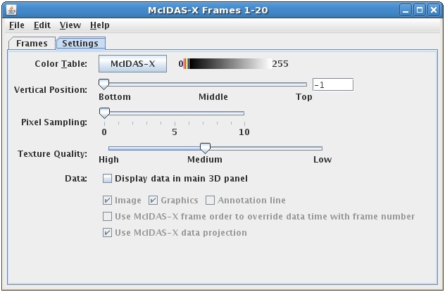
Vertical cross sections can be made in three types of displays, with contour lines, color-filled contours, and as a color-shaded image.
Controls looping of displays when more than one data time is loaded. See more in Time Animation Control.
The Grid Table display in creates a table in the Layer Controls tab of the Data Explorer. This chart plots the numerical value of your selected field at every latitude and longitude point. You can change the order of the items in this chart by Latitude, Longitude, or field values by clicking on the title of the respective column in the table. This will change the order of the table to go from lower to higher values, or higher to lower values.
All of the menu items seen utilizing this display are standard options that can be found in the Menus section of the Layer Controls page.
The Omni controls consist of a VisAD Spread Sheet, loaded with the parameter selected and its coordinates and units. The Spread Sheet is used to create a display where you have complete control over which coordinates are the axes, how it is colored, and so on. Use of the VisAD Spread Sheet is not described here. See the VisAD Spread Sheet document at https://www.ssec.wisc.edu/~curtis/ss.html.
Many of the menu items seen utilizing this display are standard options that can be found in the Menus section of the Layer Controls page. However, there is one option that is unique to this display.
The Edit menu has this unique option:
The Jython Controls allow for the development of custom layer controls written in Jython. The controls operate in two modes.
First is the "developer" mode. Here the developer can create a Jython Control; specify the name of the display, any data categories, and the probe type; and write the Jython that creates a GUI and responds to data, animation time and probe position changes.
The default Jython code has examples of accessing data, etc.
The second mode is "user" mode. In developer mode you can write out an specification of the Jython Control to a plugin through the File->Save->Write to Plugin menu. This plugin, when loaded, will only show the user interface that is created by the developer-written Jython.
The Contour Properties Editor is invoked from any contour display control with the Contour: Change button or through the Edit->Change Contours... menu item in the Layer Controls tab of the Data Explorer. Use the items in this window to set contouring properties.
The Properties dialog is accessed by right clicking on a layer in the Legend of the Main Display window, and selecting Edit->Properties menu item. This dialog can also be accessed in the Layer Controls tab of the Data Explorer, by clicking the ![]() button at the bottom of the tab. The Properties dialog consists of a Settings tab, and possibly others depending on item being displayed:
button at the bottom of the tab. The Properties dialog consists of a Settings tab, and possibly others depending on item being displayed:
There may be other tabs shown, depending on the display. For example, the Color Scale tab allows for the configuration of where the color scale bar is shown. The Spatial Subset tab allows for defining further spatial subsetting of the data.
For those controls that include color tables, the color scale can be displayed in the Main Display window. Use the the Edit->Properties->Color Scale menu in the Layer Controls tab of the Data Explorer to configure the visibility, positioning, and labeling of the color scale.
There are many different sources of data that can make use of the charting facility in McIDAS-V. It is possible to use the charting facility to display your data by selecting Data Probe/Time Series in the Displays menu in the Field Selector tab of the Data Explorer. The chart will be plotted in the Layer Controls tab, while a square representing the location of the probe will be shown in the Main Display window. The location of the probe can be changed by left-clicking on the probe and dragging it.
There are four levels of configuration available to the user, as well as several unique menu options for this display.
At the lowest level, you can set the properties of how each parameter or field is shown. This is done through the Chart Line Properties dialog, which is opened by right-clicking on the parameter below the chart and selecting Chart Properties.
For each individual plot, there are a number of settings that can be changed through the Plot Properties dialog. This is also accessed through the View->Chart->Chart:->Properties... menu item.
When right-clicking on a chart, you can also zoom in and out and save the chart as an image. There are also a number of key and mouse bindings on the chart:
When you have multiple charts, you can define different layouts for them using the View->Chart->Layout menu item. There are a number of pre-defined layouts: Grid, Vertical, Horizontal, 2 Column, 3 Column, Tabs. The Grid Layout allows for much flexibility in how the charts are organized and laid out. The View->Chart->Layout->Change Grid Layout menu item brings up the Grid Layout Editor:
You can add/remove rows and columns with the ![]() buttons.
You can then drag the graphical representations of the charts to place
them in the grid. A chart can also span multiple rows or columns. This is done by grabbing the
black square on one side of the chart image and dragging it to change the
row or column.
buttons.
You can then drag the graphical representations of the charts to place
them in the grid. A chart can also span multiple rows or columns. This is done by grabbing the
black square on one side of the chart image and dragging it to change the
row or column.
Many of the menu items seen utilizing this display are standard options that can be found in the Menus section of the Layer Controls page. However, there are several menu options that are unique to the Data Probe/Time Series display.
The File menu has these unique options
The Edit menu has these unique options:
The View menu has these unique options:
The Ensemble Grid feature in McIDAS-V allows you to create a plot of possible forecast scenarios from model data. This plot is produced by adding a perturbation to the initial model solution, and by adding perturbations to every subsequent perturbation. Thus, each perturbation away from the unperturbed initial model output theoretically diverges further from the initial model solution. These perturbations can be the result of slightly different initial conditions or different physics utilized by the model. Ensemble Grid displays are a valuable tool for medium range weather forecasting.
The Ensemble Grid controls are accessed through the Data Explorer window by selecting an ensemble run in the Data Sources tab, and then defining the parameter to display and the output format in the Field Selector. You can also utilize McIDAS-V's ensemble formulas to display this data.
By default, McIDAS-V displays all ensemble members. This can be changed in the Field Selector by selecting the Ensemble tab. You can select a range of ensemble members with the Shift key, or individual ensemble members with the Ctrl key. The times used to display the data can be changed in the Times tab. When displaying a 3D grid parameter, use the Level tab to select which level(s) to display. You can select a specific region to plot the data with the Region tab, or select how many data points to plot with the Stride tab. Press ![]() to plot the data in the Main Display window.
to plot the data in the Main Display window.
There are a variety of ways to customize the display once it has been plotted. These options can be found in the Layer Controls tab of the Data Explorer.
Many of the menu items seen utilizing this display are standard options that can be found in the Menus section of the Layer Controls page. However, there are a couple of options that are unique to this display.
The Edit menu has this unique option:
The View menu has this unique option:
This section describes:

This menu lists the recently accessed data sources and layers and allows you to easily load them. This includes data sources from your current McIDAS-V session, and from previous sessions.
This menu lets you manage and load your favorite bundles.Below the main menus you will find the main toolbar of the Main Display window.

Many of the more commonly used features of McIDAS-V can be accessed here. Hold your mouse over a toolbar button to get a popup tip on what that button does. The main toolbar is user configurable. Right-click on the toolbar to change the icon sizes and select "Customize..." to open the User Preferences' Toolbar Options tab where you can add, remove, and change the position of the buttons in the toolbar.
You can also undock the main toolbar from the Main Display window by left-clicking and dragging the textured area on the left side of the toolbar. This will place the main toolbar in its own window. To dock the toolbar back into the Main Display window, click the 'x' in the toolbar's window.
McIDAS-V has drag and drop tabs which allow you to organize multiple tabs and windows.
Drag and drop tabs allow you to separate tabs into individual windows, combine windows into tabs, as well as reorganize the layout of tabs in a window. Drag tabs into separate windows by using the left-click and drag option to drag the tab outside of the Main Display window. When the last tab in a window is moved into another window, the window will disappear. When tabs are rearranged or added from a different window, green arrows will point to the location the new tab will be placed.
Rename the tab by double clicking on it. Close a tab by clicking on the
![]() on the right side of the tab. Closing a tab will remove all layers associated
with the display, but will not remove the data sources.
on the right side of the tab. Closing a tab will remove all layers associated
with the display, but will not remove the data sources.
The View and Projections menus are associated with the 3D display and are located in the Main Display window.
The View menu lists the displays shown in this window, allows you to change the point of view, capture images and movies, and make some other changes to the overall display.
The formats include:
Accessed through the View->Properties menu item in the Main Display window, this Properties dialog allows you to control many aesthetic aspects of the display. The Properties dialog window is composed of five tabs: Main, Aspect Ratio, Lighting, Vertical Scale, and Horizontal Scale. If you are working with a globe display, there is no Horizontal Scale tab, but there is an additional tab for Globe Background.
The Main tab of the Properties dialog allows you to change several general settings pertaining to the display. Many of the items in this tab can also be found in the Display Window tab of the User Preferences window.
The Aspect Ratio tab of the Properties dialog allows you to change the aspect ratio of the display with respect to the X, Y, and Z directions. You can change the individual X, Y, and Z values by using the slider. Any changes will be made to the display once you hit Apply or OK. The Display Matrix Settings panel will actively update as you change the X, Y, and Z values, and as you rotate or zoom in/out of the Main Display window.
The Lighting tab of the Properties dialog allows you to add the effect of light shining on your display from different angles along the X, Y, and Z axes. The default values are listed in the image below.
The Vertical Range tab of the Properties dialog allows you to change the vertical scale used for the Z-axis of the display in the Main Display window.
The Horizontal Scale tab of the Properties dialog allows you to set the visibility and properties of the latitude/longitude labels along the outside of the wireframe box.
The Globe Background tab of the Properties dialog allows you to set the color and the vertical positioning of the globe background. Note that you must have the Show Globe Background option in the Main tab of the Properties dialog selected to use the globe background. This tab is only available if you are using a Globe Display.
In the Legend of the Main Display window, the Layer Visibility checkbox to the left of each layer's label can be used to toggle the visibility of that layer. This checkbox can also be selected in the item's Layer Controls tab by selecting View->Visible. Visibility animation cycles through the visibility of each layer, showing them one at a time. This is not a time animation loop; it loops through the visibility of the layers present in the Main Display window.
The padlock icon  on the right side of each layer in the Legend is used to block the effects of the visibility animation described above. When locked (
![]() ), the visibility of the layer is not affected by the animation.
), the visibility of the layer is not affected by the animation.
Visibility Animation can be invoked via the Layer Visibility Animations button. You can add this button to your main toolbar in the Toolbar Options tab of the User Preferences window.
You can also access this tool in the Main Display window through the View->Displays->Visibility Animation menu item. In this menu, you can turn visibility animation on/off, and change the speed of the animation.
As an alternative to the Layer Visibility Animations tool, the function keys F1, F2, F3* can be used to cycle visibility as follows:
Each McIDAS-V display area has a set of time animation controls above the Main Display window.
The Time Animation Widget controls looping of displays through time. A series of small green boxes is displayed representing each frame of the animation. The box corresponding to the current time is colored blue. Click on a box to select a different time. Right-click on a box to disable that frame in the animation. Disabled boxes will be colored red. You can also Ctrl+left click on a box to turn on/off all of the frames to the left of the box you clicked on, and Shift+left click to turn on/off all of the frames to the right of the box you clicked on.
The time of the data is displayed in the labeled pull-down list and in the entries of the pull down list on the left. Holding the mouse over the time will show information about how many frames are in the loop, and what the starting and ending times are. The toolbar of button icons, on the right, control time animation. The Time Animation Widget buttons do the following:
Click on the  in the animation controls to see the Time Animation Properties Dialog box. This dialog has two tabs: Settings and Define Animation Times.
The Settings tab allows you to define how looping will work for your display:
By pressing ![]() or
or ![]() , you
will set the properties in the Animation Widget. If you have the Save
As Default checkbox checked, then the properties will be saved and
used every time a new Animation Widget is created. For example, you may find
that you are always setting the dwell rate to a particular value. You can save
that state as the default state for all Animation Widgets that are subsequently
created, both in the current run of McIDAS-V and in future runs.
, you
will set the properties in the Animation Widget. If you have the Save
As Default checkbox checked, then the properties will be saved and
used every time a new Animation Widget is created. For example, you may find
that you are always setting the dwell rate to a particular value. You can save
that state as the default state for all Animation Widgets that are subsequently
created, both in the current run of McIDAS-V and in future runs.
 to change the values or type a value into the field and press Enter. Values are seconds/frame.
The Define Animation Times tab allows you to define a custom animation time set:
By default, the times used in the animation time set are all of the times from the data that is being displayed. However, you can define your own time set by selecting the Define your own list of times button.
You define how to determine the start time, end time and a time interval. The time interval is used to create the set of time steps (inclusive) between the start and end times. The start time and end time modes are determined one of four ways:
Once you select the start and end time modes you can define an offset which is
added (or subtracted) to the base time. To change the offset select the  button.
When you do this the Offset dialog will be shown:
button.
When you do this the Offset dialog will be shown:
This allows you to define a time offset by entering years, days, hours and minutes. Note that this Offset dialog will also include a +/- option when selected from Start Time or End Time.
The ![]() button gives you another way to adjust the items in the Define Animation Times tab. The two options from this button are Uniform Across Data Range and Real Time.
button gives you another way to adjust the items in the Define Animation Times tab. The two options from this button are Uniform Across Data Range and Real Time.
The Legend in the Main Display window lists the set of Layer Controls within that view. The Legend can be floated from the Main Display window. This is done with the ![]() Float Window button (the
Float Window button (the ![]() Embed Window button will move the Legend back into the Main Display window).
Embed Window button will move the Legend back into the Main Display window).
The Legend shows each layer under the Layer Category of that display. For example, the Legend in the above image shows the categories "Maps", "Radar Displays", and "Plan Views". The Layer Category may be changed. This is useful for grouping and controlling the visibility of a group of layers.
The Legend Label shows the parameter or Field name, the display type, and sometimes other information such as the level of a plan view or value of an isosurface. The label may be changed using items under the Edit->Properties menu item. Clicking on the blue, highlighted part of the label will bring up the Layer Controls tab of the Data Explorer. Right-clicking will allow you to open the Layer Controls tab for that parameter, or access the menu options in the Layer Controls tab.
Each layer category within the Legend can be toggled to show or hide the layers under that category with the Toggle Category button. The visibility of the layers under a category (e.g., Radar Displays, Plan Views, etc.) can be changed with the Category Visibility checkbox. The visibility of an individual layer can be changed with the Layer Visibility checkbox.
The ![]() Remove button quickly removes a layer. The
Remove button quickly removes a layer. The ![]() Visibility Toggle Lock "locks" the current visibility of the layer and does not change it while cycling visibilities.
Visibility Toggle Lock "locks" the current visibility of the layer and does not change it while cycling visibilities.
Detailed information about a layer may also be shown in the Legend. For example, for those layers that use a color table, the color bar will also be shown in the Legend. Moving the mouse over the color bar shows intermediate values. Right-click on the color bar to open the Color Table Editor, change the range, select other color tables, etc. You can also modify the color bar interactively for each display.
Click the color bar in the Legend to interactively modify the color bar. Holding the cursor over the color bar shows the interactive color bar editor instructions.
These controls are activated once the color bar is clicked on in the Legend.
At the bottom of the Main Display window is a status bar. This bar is useful for seeing how much memory has been used, the current time, what McIDAS-V is doing, as well as the value of the parameter probed in the Main Display window. You can change the panel on the left back and forth between displaying time or memory by left-clicking on the time or memory that is currently being displayed.

The time displayed in the left panel of the status bar is not the time associated with the data you have loaded into McIDAS-V, but rather the current time in GMT.
The memory displayed in the left panel of the status bar is in the format of (Currently used memory)/(Max used memory thus far in the session)/(Max memory available for McIDAS-V to use) in MB. You can change the amount of memory allocated by McIDAS-V at startup in the Advanced tab of the User Preferences window. When McIDAS-V has used up the majority of its available memory, the memory panel of the status bar will turn pink and then red. This will cause McIDAS-V to slow down, and may eventually prevent new data sources from being loaded. You can mitigate this problem by right-clicking on the memory and selecting: ![]() . This will clear out some memory so you can still work efficiently in your current session.
. This will clear out some memory so you can still work efficiently in your current session.
To the right of the Time/Memory readout panel is a Messages readout panel that tells you what McIDAS-V is doing. If no data is being loaded or no data sources are being loaded into McIDAS-V, this panel will be reserved for displaying the Latitude, Longitude, and Altitude information at the location of your cursor over the Main Display window. In the example above, a Grids data source is being loaded from an OPeNDAP server. If you are loading data into McIDAS-V as a loop, the middle message panel will list the data source name and also indicate how much data has loaded. To the right of this message is a loading panel. When data is loading into McIDAS-V, you will see this blue bar move from side to side. When McIDAS-V is completing various processes, different messages may be overlaid on top of this loading bar, including "Reading Data" and "Creating Layers".

As a default in the Navigation Controls tab of the User Preferences window, holding down the middle mouse button over your display will probe the data and give a numerical readout of your displayed parameter(s). The probe value(s) will be listed at the bottom of the Probe Readout panel. This panel also lists the location of your mouse when you probe the data with respect to Latitude and Longitude. As a default, this panel will list your data source and the display type. You can change how your data source will be labeled in this panel by right-clicking on the item in the Legend, and going to Edit->Properties.... In the Settings tab of this Properties dialog, you can change the Legend Label to say anything, including adding macros to further customize the readout in this panel.
There are several methods to zoom, pan, and rotate in McIDAS-V. You can use the mouse, the arrow keys, a rubber band box, or the Zoom/Pan Toolbar. To reset to the initial base viewpoint use the key combination Ctrl+R.
Note: You need to click in the Main Display window when using key combinations.
Note: If you are using an Apple Mac with a single button mouse, see Apple Mac One Button Mouse Controls.
| Mouse | ||
| Shift-Left Mouse Drag: Select a region by pressing
the Shift key and dragging the left mouse button (MB1). Shift-Right Mouse Drag: Hold Shift key and drag the right mouse button (MB3). Moving up zooms in, moving down zooms out. |
Ctrl-Right Mouse Drag: Hold Control key and drag right mouse to pan. | Right Mouse Drag: Drag right mouse to rotate. This works for a globe display. |
| Scroll Wheel | ||
| Scroll Wheel-Up: Zoom out. Scroll Wheel-Down: Zoom in. |
Ctrl-Scroll Wheel-Up/Down: Rotate clockwise/counter
clockwise. Shift-Scroll Wheel-Up/Down: Rotate forward/backward clockwise. |
|
| Arrow keys | ||
| Shift-Up Arrow: Zoom in. Shift-Down Arrow: Zoom out. |
Ctrl-Up arrow: Pan down. Ctrl-Down arrow: Pan up. Ctrl-Right arrow: Pan left. Ctrl-Left arrow: Pan right. |
Left/Right Arrow: Rotate around vertical axis. Up/Down Arrow: Rotate around horizontal axis. Shift-Left/Right Arrow: Rotate clockwise/counter clockwise. |
The default mouse and keyboard controls can be customized using the User Preferences window's Navigation Controls tab by selecting Edit->Preferences from the main menu.
Mouse controls are a bit more challenging if you are running McIDAS-V on a Mac with a single mouse button. The typical left mouse button (MB1) functions are done with a click of the button. Right mouse options (MB3) are simulated using the Option key with a mouse click. Use the following:
There is no replacement for the mouse panning actions on the Mac. Use the keyboard arrow functions or the Viewpoint toolbar instead.
The Viewpoint Toolbar allows you to quickly switch between different viewpoints, change the perspective of the display, and add rotation.
The Zoom/Pan Toolbar assists in navigating the 3D space.
The Viewpoint Undo/Redo buttons allow you to undo/redo any zoom/pan/rotation/projection change made to the display. Note that you can hold down Shift and click these buttons to go forward/back 10 changes at once.
The Transect View is a 2-Dimensional display that shows data along a transect line. This type of view can be created through the File->New Display Tab(Window)->Transect Display menu item in the Main Display window.
The left vertical axis shows altitude in meters, the right axis shows pressure levels. The bottom horizontal axis shows distance along the transect. The top horizontal axis shows the latitude and longitude locations of the end points of the transect line drawn in the map display. You can zoom and pan in this display with the normal key and mouse combinations. The transect display will also be duplicated in the Layer Controls tab of the Data Explorer.
To work with a transect display, you must have two tabs/windows open. One of these tabs/windows must have the transect display, and the other must have a standard map display. To control the location of the transect, in the transect display tab, select Transects->Edit. This creates a Transect Drawing Control in the map display. Using the Create a transect Mode, click and drag in the map display to draw the transect. The transect drawn in the transect display will be representative of the most recent transect line you have drawn. You can also select any of the pre-defined or user created transects from the Transects menu of the transect display.
In the Transects tab of the Properties dialog for the Transect View (from View->Properties menu item in the transect display window/tab) you can define a maximum distance to show. Normally, data that lies with the bounding lines that are orthogonal to the transect line is shown in this display. The max distance gives a display radius. Data that lies past this max distance is not displayed.
This section contains information about the different display controls that you can utilize in McIDAS-V. All of these display controls can be found in the menus of the Main Display window.
The range rings control displays a set of concentric circles labeled by distance from the central point, with radial lines, useful for judging distance and angle from a geographic location. You display range rings from the Main Display window with the Display->Add Range Rings menu item. Range rings are often used with radar imagery, but they can be used with any data. The control window is composed of two tabs: Location and Settings.
The Location tab allows you to specify the location to center the range rings:
The Settings tab allows you to control how the range rings are displayed:
The range rings are oriented with local north-south on the displayed map projection. In some cases, the eastward radial line may not be horizontal. The range rings will appear centered on the map projection. You can move the range rings by resetting the latitude-longitude or the station. McIDAS-V can display multiple range rings at once and at any location.
Many of the menu items seen utilizing this display are standard options that can be found in the Menus section of the Layer Controls page. However, there is one option that is unique to this display.
The Edit menu has this unique option:
The Range and Bearing Controls show the distance, azimuth, and back azimuth of a great circle line connecting two positions on the Earth's surface. This feature can be found in the Main Display window in the Display->Add Range and Bearing menu item.
When the range and bearing controls are first created, a range and bearing line is added to the Main Display window. The distance, azimuth, and back azimuth values are shown on the Legend and at the top of the Range and Bearing control window. The latitude/longitude position values of the endpoints are shown in the control window. Computations are based on the WGS-84 reference ellipsoid, using computation code from the U.S. National Geodetic Survey. You can reposition the endpoints by left-clicking and dragging them in the Main Display window, entering new values into the Latitude/Longitude boxes in the control window and pressing Enter or clicking ![]() , or selecting a location in the dropdown menu to the right of the Latitude and Longitude fields.
, or selecting a location in the dropdown menu to the right of the Latitude and Longitude fields.
Note The line shown on the display is not the great circle path connecting the end points. The values are computed for a great circle path on the ellipsoidal Earth, using the numerical latitude and longitude values, not the line on the display. The line shown in the display is a straight line on whatever map projection you happen to have; usually it will not coincide with the great circle line.
Note If you change the map projection, an existing range and bearing map line will stay at the same location in the display, hence the end points on the map are in new locations. The distance, azimuth, etc. values in the control window reflect the latitude-longitude positions in the control window and hence do not match the display picture until an end point is moved by hand.
Many of the menu items seen utilizing this display are standard options that can be found in the Menus section of the Layer Controls page. However, there are a couple options that are unique to this display.
The Edit menu has these unique options:
The transect drawing controls are a version of the Drawing Controls that allows you to view, create, and modify the transect lines that are used in the Transect Views. This option can be found in the Main Display window under the Display->Draw Transect menu item or through the Transects menu in the Transect View.
This display control is a representation of the set of transects that are defined by the transect resource. Not only does it have its own state (that can be saved in a bundle, for example), but it also writes out any transects you may create or change into your local McIDAS-V state directory in a transects.xml file. This transects.xml file (if one is created) is carried over from session to session. Therefore, if you draw transects in one session and save the transects (via the File->Save or Automatically update transects items), the same transects will appear in subsequent sessions when you open the Transect Drawing Control widget.
In this control, there is only one shape that you can draw, a Transect Line. This control also shows a non-editable Transect Shape which displays the full transect line used by any Transect Views, called the "Active Transects". There are also a set of transect lines that are non-editable that are from the system transects property. For an active transect, if the Transect View that it represents has a max distance set then the transect will show this max distance as a rectangular box.
The Transect Drawing Control window consists of three tabs: Controls, Style, and Shapes.
The Controls tab allows for the user to draw features in the Main Display window:
 Select - Allows you to select one or more transect drawings. To select multiples press the control key. The selected transects will be shown with small magenta rectangles. Once selected you can bring up the transect's property editor by pressing Ctrl+P. You can also delete the selected objects by pressing Ctrl+X. You can select all of the objects by pressing Ctrl+A.
 Move or stretch graphic - Allows you to reposition a transect without stretching (changing the distance between the endpoints) it.
 Stretch Graphic - Allows you to move one of the endpoints of a transect. The other endpoint will remain in its fixed location.
The Style tab controls the appearance of the transect lines in the Main Display window:

These menu options apply to the shapes listed in the Controls tab. Once modifications have been made in this tab, they will be applied to the next transect you draw in the Main Display window, without changing any transects already created. Note that Font and Justification are not valid options for this control, since there is no text component in the Controls tab.
The Shapes tab lists all of the graphical elements:
Double-clicking on an element in the Shapes tab will show its properties editor, which consists of two tabs: Properties and Points.
The Properties tab gives general information about each transect:
The Points tab gives general information about each shape:
You can modify a latitude/longitude value here by double-clicking in one of the cells for latitude or longitude, entering a new value, clicking in another cell, and clicking Apply or OK. The new latitude/longitude values will be applied to the endpoints of your transect line in the Main Display window.
Many of the menu items seen utilizing this display are standard options that can be found in the Menus section of the Layer Controls page. However, there are several options that are unique to this display.
The File menu has these unique options:
The Edit menu has these unique options:
The drawing controls consists of a drawing editor that supports polygons, lines, shapes and text. This tool allows you to create and move graphics in the Main Display window. Drawing and selecting in 3D can be difficult and sometimes it is best to be in the main overhead view. This feature can be found in the Main Display window in the Display->Draw Freely menu item.
The Drawing Control window consists of three tabs: Controls, Style, and Shapes.
The Controls tab is used to draw features in the Main Display window:
 Select - Selects one or more drawing objects. To select multiples press the Control key. The selected objects will be shown with small magenta rectangles. Once selected, you can bring up the object's property editor by pressing Ctrl+P. You can also delete the selected objects by pressing Ctrl+X. All of the objects can be selected by pressing Ctrl+A. Move - Activates and moves the active object (the object with pink squares at its corners/along the line). Do this by left-clicking and dragging the object. Reshape - Stretches an object drawn in the Main Display. To use this, left-click and drag on a pink square of an active object. As you move this point, other points in the object will move as well to keep the object smooth.
 Create a polygon - Creates a smooth polygon.
 Create a rectangle - Creates a rectangle.
 Create a diamond - Creates a diamond.
 Create text - Opens a Text entry window, where you can type in text or HTML. Click OK when done, and the text will appear in the Main Display window.
 Create waypoint - Opens a Text entry window, where you can type in text or HTML. Click OK when done, and the text will appear in the Main Display window along with a marker to represent the exact location where you clicked in the Main Display window.
 Create image - Places a saved image or an image from an HTML address on the Main Display window. Select an image file from the file chooser or enter a URL. When using this shape, you can use the Full Lat/Lon option next to Coordinates. This controls how the corners of the image are positioned. If you are adding a large image and you want to display the full image right away without having to stretch it, check this option. Otherwise, your image will be compressed in the horizontal.
 Create quicktime movie - Places a movie on the Main Display window. Select the movie from the file chooser or enter a URL. This can only work with certain types of Quicktime (*.mov) files.
 Create a symbol - Places a cross (+) symbol on the display. This symbol can be changed in the Properties Editor of the shape. You can get to this through the Shapes tab of the Drawing Control and double-clicking on the item. Use the Symbol button to change the symbol to a variety of meteorological symbols including various types of weather conditions, clouds, and turbulence.
The Style tab controls the style that the drawings take in the Main Display window:
These menu options apply to the shapes listed in the Controls tab, excluding the High/Low pressures/fronts. Once modifications have been made in this tab, they will be applied to the next shape you make in the Main Display window, without changing any shapes already created.
The Shapes tab lists all of the graphical elements:
This tab lists out the different shapes drawn in the Main Display window from the Controls tab, as well as other information about them.
Double-clicking on an element in the Shapes tab will open its Properties Editor, which consists of two tabs: Properties and Points.
The Properties tab gives general information about each shape:
This tab allows you to control many aspects of the individual shapes. After making any modifications to this window, click Apply or OK, and the changes will be applied to the shape in the Main Display window. Note: The different types of shapes will have different menu options.
The Points tab gives general information about each shape:
This tab lists out location coordinates of your shape. The points listed can be seen in the Main Display window, and are represented by the pink squares along the boundaries of the shape. These values can be changed by double clicking on a coordinate, and typing in a new value. Once you click on a different coordinate, and then press Apply or OK, the change will be made in the Main Display window.
Many of the menu items seen utilizing this display are standard options that can be found in the Menus section of the Layer Controls page. However, there are several options that are unique to this display.
The File menu has these unique options:
The Edit menu has these unique options:
The location indicator controls display a configurable axis in the Main Display window and (optionally) a bearing point. This option can be found in the Main Display window under the Display->Add Location Indicator menu item. The Location Indicator window consists of three tabs: Location, Settings, and Orient.
The Location tab displays and allows you to modify the position of the origin and the bearing point:
The center point of the Location Indicator can be moved by left-clicking and dragging on the lines produced in the Main Display window. You can also move the center point of the Location Indicator with a series of Ctrl+Alt key combinations.
The Settings tab allows for the configuration of display settings:
The Orient tab allows for the orienting the display based on the location. To change the origin, click and drag in the main display. To show and/or change the bearing point, do a Control+drag in the Main Display window. The x/y/z locations of the bearing point are shown on the origin axis as tick marks and, optionally, as longitude/latitude/altitude readouts:
Many of the menu items seen utilizing this display are standard options that can be found in the Menus section of the Layer Controls page. However, there are some options that are unique to this display.
The Edit menu has this unique option:
The View menu has these unique options:
The WMS Controls display imagery from WMS servers. A set of predefined links to WMS servers for topographic, shaded relief and aerial imagery is also provided with the Background Image control.
To use the pre-defined background images, in the Main Display window, select the Display->Add Background Image menu item. To choose imagery from web map servers, bring up the Catalog Chooser in the Data Explorer and enter the URL that points to the Capabilities document of the desired WMS. We also provide links to a set of useful WMSs from the idvcatalog. If it is not in the Catalog pull down menu, enter the following url:
http://www.unidata.ucar.edu/georesources/idvcatalog.xml
From this catalog open the Web Map Servers tab and select the WMS you would like to access.
The WMS Controls makes a request to the Web Map Server for an image that covers the area currently being displayed in the Main Display window. Due to the time it takes to access remote servers, the WMS Control does not request new images while the user pans and zooms.
 Reload the image - Reloads the image from the server at the current screen location.
  Reproject to image - Sets the projection in the display to the current image bounds.
 Many of the menu items seen utilizing this display are standard options that can be found in the Menus section of the Layer Controls page. However, there are several options that are unique to this display.
The File menu has this unique option:
The View menu has these unique options:
McIDAS-V can display QuickTime movies. You can pause, single step and play a movie. This option can be found in the Main Display window under the View->Capture->Movie menu.
The media properties is composed of three tabs, General, Video, and Plug-in Settings.
The General tab has general information about the QuickTime movie:
The Video tab lists the specific video information:
The Plug-in Settings tab has access to the PlugIn Viewer details:
All of the menu items seen utilizing the movie display are standard options that can be found in the Menus section of the Layer Controls page.
You can capture the Main Display window as an image, a QuickTime movie or an animated GIF.
You can save a display as an image by selecting the View->Capture->Image... menu item in the Main Display window. A file dialog will open where you can enter a file name for the image file. McIDAS-V supports JPEG, PNG, GIF, PDF, PS, and SVG formats. From this File Dialog you can also specify the image quality (only used for JPEGs) and what to capture. You can also select whether or not the background is transparent.
Note: When capturing an image, the Main Display window cannot be obscured.
McIDAS-V can also write out an image and the corresponding Google Earth KML or KMZ file. For this to be correct, the projection must be a Lat/Lon geographic projection (i.e., rectilinear) and in an overhead view. Some of the default projections that are Lat/Lon include World, Africa, Asia, Australia, and the individual state projections (US->States->...). You can also create your own Lat/Lon projection using the Projection Manager. The simplest way to get a correct projection is to select the Projections->Use Displayed Area menu item in the Main Display window. If you specify a .kml file, McIDAS-V will generate an image with the same file prefix and the kml file that refers to the image. If you specify a .kmz file (which is a zip format) it will contain the image and the kml file.
You can send any display to a printer. Select the View->Capture->Print... menu item in the Main Display window. A Print dialog will popup where you can configure and print an image.
You can save any sequence of displays as a movie. Select the View->Capture->Movie... menu item in the Main Display window to open the Movie Capture window:
Note: More information about these controls is found in the Creating a Movie section below.
To make a movie, there are three steps: capturing the frames, previewing the frames, and creating the movie. McIDAS-V supports QuickTime movies, animated GIF and AVI files, Google Earth KMZ and AniS or FlAniS HTML file formats.
McIDAS-V supports displaying certain types of QuickTime movies (including the ones McIDAS-V generates). These movies can be loaded in the General->Files/Directories Chooser in the Data Sources tab of the Data Explorer.
McIDAS-V makes use of a timeline widget in a variety of areas. The timeline allows you to see the temporal distribution of a set of times and easily select them. There can also be a date selection mechanism (see below) that allows you to select based on a range, interval, etc.
The date selection settings can be accessed by right-clicking in the timeline to show a popup menu. The menu allows you explicitly define these settings through a Properties dialog or set them directly with sub-menu choices. The date selection settings are listed below.
The View Managers use the timeline to show the animation time set and the times of the different displays. Here, the timeline is used for informational purposes and is not used to select times. This can be shown through the View->Animation Timeline menu. The gray timeline represents non-visible displays. Double clicking in a timeline sets the animation step to that time.
The timeline supports a variety of navigation mechanisms:
| Event | Action |
| Left Mouse Drag | Change visible range or date selection range. |
| Left/Right Arrow | Change visible range. Use Ctrl+Key to change date selection. Use Shift+Key to use larger increment. |
| Up/Down Arrow | Zoom in/out visible range. Use Ctrl+Key to change date selection. Use Shift+Key to use larger increment. |
| Mouse Click; Control-Click; Shift-Click | Select individual times, multiple times or a range of times |
| Shift-Drag | When not showing the date selection mechanism you can choose a range of times with shift-drag |
| Right Mouse Click | This brings up a popup menu that allows you to show the properties dialog, go to particular current date ranges, set the interval, range, skip factor and count of the date selection. |
Preferences are used to save standard settings of McIDAS-V, such as the map projection to show when McIDAS-V starts. The Preferences Dialog is opened in the Main Display window through the Edit menu with Edit->Preferences.
Click on Cancel if you wish to exit preferences setting, Ok to accept the changed preferences and close this window, and Apply to accept the preferences and keep this window open.
Note: Some of these preferences only take effect the next time you run McIDAS-V or when you create a new view window. The preferences also may be overwritten when you use bundles.
The follow sections describe the different user preference options for McIDAS-V:
The User Preferences window is accessed in the Main Display window through the Edit->Preferences menu. The General tab allows the user to configure many of the general settings within McIDAS-V. The image below represents the default settings for the General tab.
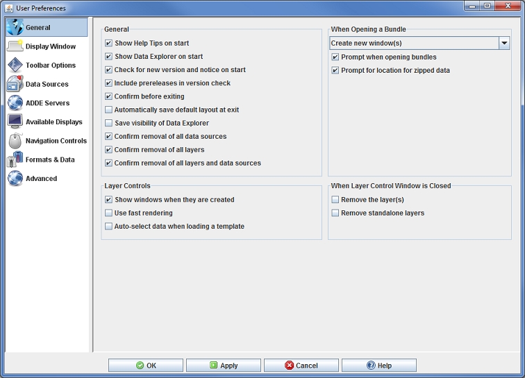
The User Preferences window is accessed in the Main Display window through the Edit->Preferences menu. The Display Window tab allows the user to set preferences related to the Main Display window. The image below represents the default settings for the Display Window tab.
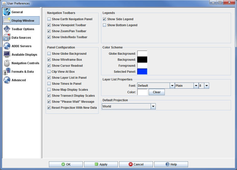
Navigation Toolbars
The User Preferences window is accessed in the Main Display window through the Edit->Preferences menu. The Toolbar Options tab allows the user to define what actions/icons are displayed in the toolbar. The list on the left shows all of the available actions. The list on the right shows the actions that make up the toolbar. The image below represents the default settings for the Toolbar Options tab.
The User Preferences window is accessed in the Main Display window through the Edit->Preferences menu. The Data Sources tab allows the user to define what types of data choosers to use. This is a way to simplify the Data Explorer window by only showing the choosers that you want to use. Note that you must restart McIDAS-V for any changes made in this tab to take effect. The image below represents the default settings for the Toolbar Options tab.
The User Preferences window is accessed in the Main Display window through the Edit->Preferences menu. The window is also accessible
by clicking the Manage servers button (![]() ) next to the server name of the
applicable choosers in the Data Sources tab of the Data Explorer. The ADDE Servers tab allows the user to add and manage a list of active ADDE servers separated by data type. The selected ADDE entries will be included in the list of servers in the Data Sources tab of the Data Explorer. Limiting the number of servers in the Data Sources tab will make it easier to find the desired sources of data.
) next to the server name of the
applicable choosers in the Data Sources tab of the Data Explorer. The ADDE Servers tab allows the user to add and manage a list of active ADDE servers separated by data type. The selected ADDE entries will be included in the list of servers in the Data Sources tab of the Data Explorer. Limiting the number of servers in the Data Sources tab will make it easier to find the desired sources of data.
The list of ADDE Servers is hierarchial, meaning that you can turn off all servers, specific groupings of servers (ex. Point), or individual servers within a group (ex. adde.ucar.edu/RTPTSRC can be turned off under POINT, but the rest can remain selected).
The image below represents the default settings for the for the ADDE Servers tab. All of the ADDE entries are checked on except for 'NAV' and 'UNKNOWN'.
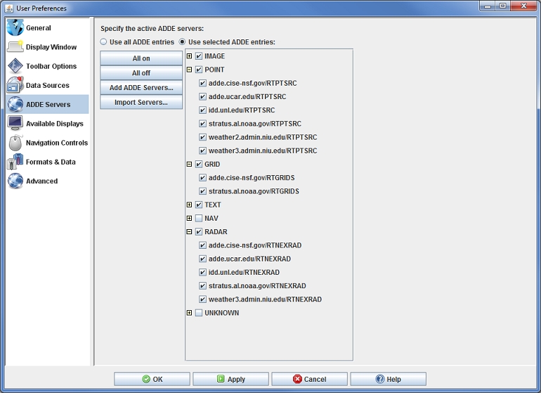
The User Preferences window is accessed in the Main Display window through the Edit->Preferences menu. The Available Displays tab allows the user to specify what types of displays to use. The chosen displays can possibly be included in the Displays list in the Field Selector if the field you are displaying incudes the display type in its properties. Choosing what displays you want to appear in the Field Selector will limit the number of displays in the list, making it easier to create your desired image.
The list of display types is hierarchial, meaning that you can turn off all displays, specific groupings of displays (ex. Plan Views), or individual display types within a group (ex. Color-Shaded Plan View can be turned off under Plan Views, but the rest can remain selected).
The image below represents the default settings for the Available Displays tab. Every display is selected on by default.
The User Preferences window is accessed in the Main Display window through the Edit->Preferences menu. The Navigation Controls tab allows the user to change how McIDAS-V interprets mouse and keyboard events for navigating in 3D space. The user can choose to use the navigation defaults for the IDV, VisAD, Google Earth, or create their custom navigation settings. The below images represent the default Custom settings for the mouse and keyboard in the Navigation Controls tab.
The User Preferences window is accessed in the Main Display window through the Edit->Preferences menu. The Formats & Data tab allows the user to define data formats and defaults to be used when displaying data. The below image represents the default values for the Formats & Data tab.
Formats
"MMMM" gives full month name

"MMM" gives short month name

"MM" gives  2 digit month number

"M" gives  1 or 2 digit month number
Symbol Description Presentation Example G Era designator Text AD y Year Number 1996; 96 M Month in year Text and Number July; Jul; 07 w Week in year Number 27 W Week in month Number 2 D Day in year Number 189 d Day in month Number 10 F Day of week in month Number 2 E Day in week Text Tuesday; Tue a Am/pm marker Text PM H Hour in day (0-23) Number 0 h Hour in am/pm (1-12) Number 12 K Hour in am/pm (0-11) Number 0 k Hour in day (1-24) Text 24 m Minute in hour Number 30 s Second in minute Number 55 S Millisecond Number 978 z Time zone Text and Number Pacific Standard Time; PST; GMT-08:00 Z RFC 822 Time zone Number -0800 ' Escape for text Delimiter '' Single quite Literal Note: The "yyyy" year symbol can also be written as "yy" for recent data. However, it cannot be written as "y".
Ex: The day 215 in the year 2009 would be written as "09215" yyDDD and not "9215" yDDD.
0 Digit # Digit, zero shows as absent . Decimal separator or monetary decimal separator - Minus sign , Grouping separator E Separates mantissa and exponent in scientific notation. ; Subpattern boundary Separates positive and negative subpatterns
Format Example ##0 -95 ##0.0 -94.6 ##0.0# -94.56 ##0.0## -94.563 0.0 -094.6 0.00 -094.56 0.###E0 1.04E2 000.#E0 104.6E0
%value% Formatted value %unit% Display unit %rawvalue% Unformatted value %rawunit% Original unit
The User Preferences window is accessed in the Main Display window through the Edit->Preferences menu. The Advanced tab allows for changing options that require a restart in order for them to take effect. To configure the settings before running McIDAS-V, execute the runMcV-Config command from the directory where McIDAS-V was installed (normally McIDAS-V-System) or by selecting Configure McIDAS-V in the Windows Start menu. The below image represents the default settings for the Advanced tab.
If running McIDAS-V on a multi-core machine, McIDAS-V can be configured to render individual time steps in parallel when working with a loop of data. McIDAS-V can also do remote data reads in parallel. This typically results in a 50% reduction in overall data reading and rendering time. For more information, see Parallel Rendering and Data Reading.
The Local and Remote ADDE Data Managers are accessible in the Main Display window through the Tools->Manage ADDE Datasets menu item. Click the Remote Data tab to manage access to data on other workstations, or the Local Data tab to manage access to data on your workstation. Continue below for more information about the Remote ADDE Data Manager, or go to the Local ADDE Data Manager page for more information.
The Remote ADDE Data Manager lets you add, delete or edit access to remote datasets that are available through the Satellite->Imagery chooser. You can also import a MCTABLE.TXT file that contains a preexisting set of entries for the Remote ADDE Data Manager.
The columns in the table are defined below.
At the bottom of this window, there is a status message that lets you know if local servers are running and does not affect remote servers. For more information this, please see Local ADDE Data Manager.
The four buttons at the bottom of the window are described in the corresponding section below.
The window below appears if you click the Add New Dataset button or select the File->New Remote Dataset menu in the ADDE Data Manager window.
The Add Remote Dataset window lets you add access to remote datasets so they are available through the Data Explorer.
The fields and buttons are defined below.
If you highlight an editable entry in the ADDE Data Manager window and then click the Edit Dataset button, the window and fields are the same as above, except that the window title is Edit Remote Dataset and the bottom buttons say Verify and Save Changes, Verify Changes, and Save Changes (rather than Verify and Add Server, Verify Server, and Add Server).
Note that you cannot edit any of the remote datasets that come with McIDAS-V.
If you highlight an editable entry in the ADDE Data Manager window and then click the Remove Selection button, it immediately removes the entry from the table. There is no recovery option, so if you accidentally remove an entry you need, you will have to remake the entry using the Add New Dataset button. Note that you cannot remove any of the native remote datasets that come with McIDAS-V.
The window below appears if you click the IMPORT MCTABLE... button in the Remote ADDE Data Manager window.
This window lets you import a MCTABLE.TXT file that contains a preexisting set of entries for the Remote ADDE Data Manager. For example, McIDAS-X users may have added access to many servers via the DATALOC command. Those entries are stored in the MCTABLE.TXT file, which can be imported to McIDAS-V.
The fields and buttons are defined below.
A couple of the menu items seen utilizing this display are standard options that can be found in the Menus section of the Layer Controls page. However, there are several menu options that are unique to this tool.
The File menu has these unique options:
The Edit menu has these unique options:
The Local Servers menu has these unique options:
The Local and Remote ADDE Data Managers are accessible in the Main Display window through the Tools->Manage ADDE Datasets menu item. Select the Local Data tab to manage access to image data on your workstation, or the Remote Data tab to manage access to data on other workstations. Continue below for more information about the Local ADDE Data Manager, or go to the Remote ADDE Data Manager page for more information.
The Local ADDE Data Manager lets you add, delete or edit local image datasets that are available through the Satellite->Imagery chooser when you select <LOCAL-DATA> in the Server field. Other types of data (e.g., grib or point) in local files can be accessed directly through other choosers (e.g., the General->Files/Directories chooser).
The columns in the table and buttons are defined below.
At the bottom of this window, there is a status message that lets you know if local servers are running. The Server Manager will attempt to connect to ports 8112 to 8122. When port 8112 cannot be connected to, port 8113 will be attempted, and then 8114 and so on. After these ports have been stopped or cannot be connected to, the status message will say "Local servers have been stopped". When this status message is showing, you cannot connect to any local servers. To help avoid connection problems, your firewall software must allow connections to port 8112.
To add a new local dataset entry, select File->New Local Dataset from the ADDE Data Manager menu, or click ![]() .
.
The Add Local Dataset window lets you add access to local image datasets so they are available through the Satellite->Imagery chooser. The fields and buttons are defined below.
To edit an existing entry, double click on the entry, select Edit->Edit Entry..., or click ![]() to bring up the Edit Local Dataset window. Make the needed changes and click
to bring up the Edit Local Dataset window. Make the needed changes and click ![]() (or click
(or click ![]() to discard any changes and close the window).
to discard any changes and close the window).
Many of the menu items seen utilizing this display are standard options that can be found in the Menus section of the Layer Controls page. However, there are several menu options that are unique to this tool.
The File menu has these unique options:
The Edit menu has these unique options:
The Local Servers menu has these unique options:
The Weather Text Product Control is used to display weather text products (forecasts, warnings, watches, etc.) produced by the National Weather Service and other international meteorological agencies. The Weather Text Product Display is accessed through the Main Display window via Tools->Text Data->Weather Text Products(from server). The user interface consists of three tabs, Products, Display, and Locations.
The Products tab selects and displays the text products. When a product is selected, the available stations are plotted in the Main Display window. One or more stations can be selected by clicking on the station in the Main Display window (or Ctrl+click for multiple stations). When a station is selected, the text product for that station is displayed in the Weather Text Product Display:
By default, the text product is displayed as raw text. Click on the HTML tab at the bottom of the display window to view the product in HTML.
By default, the most recent text product is displayed. Previous versions of the products can be displayed by selecting a time range from the Time Covered drop-down list. Use the Time Animation Widget to loop through multiple products. The time animation will be synced with any other data in the Main Display window.
The Display tab controls the display of the station locations in the Main Display window:
The Locations tab lists information about the selected location and shows lists of all the locations and the locations currently visible in the Main Display window:
Many of the menu items seen utilizing this display are standard options that can be found in the Menus section of the Layer Controls page. However, there are some options that are unique to this display.
The Edit menu has these unique options:
The View menu has these unique options:
The Storm Track Control displays tropical storm observation and model output tracks. Currently the McIDAS-V supports both the Automated Tropical Cyclone Forecasting System (ATCF) data as well as data from the Shanghai Typhoon Institute.
To load in ATCF data select the Tools->Text Data->ATCF Tropical Storm Data menu item in the Main Display window. This creates a data source with a predefined path to the National Hurricane Center ftp site. Then, create the Storm Track display.
The display control shows the set of available storms on the left panel organized by year and basin, e.g., Atlantic (AL), Eastern Pacific (EP) and Central Pacific (CP).
At the top of the list is an option (Yearly Tracks) which allows the user to display the observed tracks for all the storms in a given year. You can load and/or unload any number of years worth of observed tracks. The color swatch changes the color of the tracks for a given year. The Time Mode menu allows one to change the animation mode, e.g., use the year or use the storm start time.
To show the observation and all of the model results for a single storm select
the storm in the list and press the ![]() button.
You can load any number of storms but they are shown in different panels. You
can use the View->Storm Tracks menu to list out
all of the loaded storms, remove them all, etc. Once a storm is loaded it can
be removed with the
button.
You can load any number of storms but they are shown in different panels. You
can use the View->Storm Tracks menu to list out
all of the loaded storms, remove them all, etc. Once a storm is loaded it can
be removed with the ![]() icon shown in the upper right.
icon shown in the upper right.
Once a storm is loaded the first thing you should do is to specify which "Techs" (or models) to use by bringing up the control's Properties dialog Edit->Properties menu. Use Ctrl+A to select all items in the tab, the left/right arrows to remove/add an item from/to the Use column, or Delete to remove an item from the Use Column.
The Storm display panel consists of three tabs: Tracks, Table and Storm Chart.
The Tracks tab controls the display and animation of the tracks.
The Table tab shows a tabular listing of all of the observational track data and individual forecast model runs. On the left is a tree view organized by the Tech and model run time. Selecting one of the model runs will display the data in the table. The main File->Save->Export to Spreadsheet menu allows you to export the track data to an Excel spreadsheet. In the File Dialog are options to select what is to be saved.
The Storm Chart tab shows time series charts of selected tracks. Under the main Edit menu you can any number of new forecast time or forecast hour charts. The forecast time chart is based around the model run time of the selected forecasts. The forecast hour charts selects data across the different model run times, e.g., you can show the 12 hour forecast from each model run.
To do the charting of the storm track, one or more Techs need to be selected. Once selected the Forecast Hour/Forecast Time list is populated. One or more times can be selected (Ctrl+click). Each Parameter that is selected will result in a new chart shown on the right.
| 0 DB | Disturbance | |
|
1 TD |
Tropical Depression |
2 TS |
Tropical Storm |
3 TY |
Typhoon |
4 ST |
Super Typhoon |
5 TC |
Tropical Cyclone |
6 HU |
Hurricane |
Many of these menu items seen utilizing this tool are standard options that can be found in the Menus section of the Layer Controls page. However, there are some options that are unique to this display.
The File menu has these unique items:
The Edit menu has these unique items:
The View menu has these unique items:
The Color Table Editor supports editing existing color tables and creating new ones. A color table is an ordered collection of colors that is used to color a display according to a range of data values.
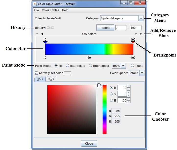
The Color Table Editor can be used stand-alone by selecting the Tools->Color Tables menu item in the Main Display window. It can also be used or in conjunction with a particular layer by right-clicking on the layer's color bar in the Legend and selecting Edit Color Table, or through the layer's Edit menu (Edit->Color Table->Edit Color Table). You can also click on the button that represents the name of the color bar in the Layer Controls tab and select Edit Color Table.
The Color Table Editor starts with a color table loaded in it. If you are working with a data display and you open the Color Table Editor through the Layer Controls tab of the Data Explorer, the color table in the editor is the same as in the display. If you want to use or edit a different color table, use the Color Tables menu to select from the categorized list of color tables:
Color tables are grouped into categories. Click on a color table to bring it into the Color Table Editor. To change to the newly selected color table for a display on the Main Display window, click OK or Apply at the bottom of the Color Table Editor. Apply will save changes to the color table, while keeping the Color Table Editor open, and OK will save any changes to the color table and close the Color Table Editor. Also, when editing a color table that is currently being used to display a layer in the Main Display window, there is an Auto update checkbox on the bottom right of the Color Table Editor. When this box is checked, any changes made to the color table will be applied directly to the display in the Main Display window. If you are making several changes to the color bar at once, and you have a lot of data displayed in the Main Display, it is recommended that you do not have this option turned on, as it will use up more memory. Once done making changes to the color bar, click Apply or OK to apply your changes to the displayed data.
You can "paint" in the color table by left-clicking and dragging the mouse within it. When your mouse is over the color table the cursor will change to a paintbrush and a gray line is drawn to indicate the position of the cursor.
The type of painting is specified by the Paint Mode buttons.
The editor uses "breakpoints" indicated along the top of the color legend with triangles and the numerical value. By default, the beginning and ending of the color bar will each be a breakpoint. You can add additional breakpoints to the color bar by right-clicking on the color bar and selecting Add Breakpoint, or by double-clicking on or above the color bar where you want a breakpoint.
Clicking on a breakpoint makes it active. The active breakpoint will have bold text for the label, and the colored triangle below it will have an outline of yellow. There is only one active breakpoint at a time. Breakpoints are used for a number of things: showing the data and transparency values at a point along the color table and changing the colors (fill, interpolation or transparency).
The values on the breakpoints are determined by the position of the breakpoint along the legend, proportional to the min and max of the Range. Changing the minimum and maximum of the Range changes the breakpoint values.
You can move the active breakpoint (assuming it isn't locked) in several ways:
If you have the Actively set color checkbox selected, when you change the color in the color chooser that color will be applied to the color slot under the selected breakpoint automatically.
You can also change colors and manipulate breakpoints by right-clicking on a breakpoint:
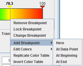
The choices are:
You can modify an existing color table, or edit an existing color table and save it with a new name to make a new color table. Any new or modified color table can be saved for future use. To save a new or modified color table simply select the the File->Save. To save a modified color table as a new color table, select File->Save As and enter the new name in the dialog box that appears. This new color table will now be permanently saved in your local collection of color tables. You can control where your color bar will be saved by selecting a Category in the upper right of the Color Table Editor.
To save a color table as a file which can be shared with others in McIDAS-V, select the File->Export menu item. A file dialog will appear that will allow you to save the color table as an XML-format file. We suggest you use a file extension of .xml.
To use a color table as a file which has been supplied to you by another McIDAS-V user, select the File->Import menu item. A file dialog will appear that will allow you to find the color table as an XML-format file. The following types of color tables can be imported:
Another way that you can save all of your color tables at once is to save them as a plugin. This can be done through the Plugin Manager, by including your colortables.xml file that is inside of your /User/McIDAS-V directory. You can then pass this on to any McIDAS-V user, and they can install this plugin and obtain all of your color bars without having to individually transfer them.
The definitions of the 3-column RGB color table are divided over a range of values. Each line represents one of the equal sized blocks on the color bar, and the bar is saved in the *.ascii format. Ascii files are text files with three space-separated columns consisting of the RGB component counts. An example is shown below:
180 0 10

140 0 50

140 0 140

80 0 180

0 120 60

0 140 80
In the example above, there are six lines (definitions) that would be divided into the color table. The color table would be broken into six even segments, with the first line applying to the first segment, the second to the second segment, etc. Your file may be any number of lines long. The values in these columns must be between 0 and 255.
The Color Chooser, in the lower half of the Color Table Editor window, allows you to select any possible color. The chooser contains two tabs, HSB (Hue, Saturation, Brightness) and RGB (Red, Green, Blue). In most cases, the HSB tab provides better control and better depiction of color changes because of its hue, saturation, and brightness controls. Thus, it is recommended that you use the HSB tab (rather than the RGB tab) unless you have specific red, green, and blue values to set.
The HSB tab allows you to control color by hue, saturation, and brightness, thereby making any color. With the HSB tab open, click on one of the radio buttons marked H, S, or B for the corresponding control for hue, saturation, or brightness. All controls in the HSB tab also show the RGB values for any color selected, in case you need to know the RGB values for another use.
Hue is the term indicating a pure color selection from the spectrum. Saturation is an indication of how much white is added to the hue. 100% saturation is pure hue with no white. Brightness is an indication of how much black is added to the hue. 100% brightness has no black and maximum brilliancy, but can be any saturation from the hue to pure white. 0% brightness is solid black. Some colors are not found in the spectrum, and are a mixture of a hue and black and/or white. You only need to use one of the controls for H, S, or B to make any color.
With the Hue (H) radio button selected, the slider bar chooses the pure hue. Once you have chosen a hue, clicking or dragging the mouse on the color display chooses degrees of saturation and brightness for that hue.
Image 6: The HSB Hue Tab, Set on Green With High
S and High B
Saturation (S) has a slider bar with the full range of saturation. The bottom is always solid black. A saturation value of 100 is the pure hue, and more black is mixed in with the hue until it is solid black at a value of 0. The saturation value can be controlled by the slider to the right of the color square, or by entering a value into the field to the right of S and pressing Enter. After selecting a saturation level, you can click and drag in the colored square to get your desired color.
Brightness (B) has a slider bar with the full range of brightness. The bottom is always solid white. A brightness value of 100 is the pure hue, and more white is mixed in with the hue until it is solid white at a value of 0. The brightness value can be controlled by the slider to the right of the color square, or by entering a value into the field to the right of B and pressing Enter. After selecting a brightness level, you can click and drag in the colored square to get your desired color.
All controls in the HSB tab show the RGB values for any color selected, in case you need to know the RGB values for another use.
The RGB tab allows you to control color by specifying individual Red, Green, and Blue components.
The individual R, G, and B components are numerically scaled between 0 and 255, ranging from black to the true color. Each color can be modified by using the slider, typing a value into the field and pressing Enter, or by using the up and down arrows to the right of the value.
As you make modifications to the RGB components, the current color will be displayed above the HSB and RGB tabs next to the Actively set color checkbox. If you have the Actively set color checkbox selected, any changes you make in this tab will be applied directly to the color bar as you make the changes.
Many of the menu items seen utilizing this display are standard options that can be found in the Menus section of the Layer Controls page. However, there are several options unique to this display.
The File menu has these unique options:
The Color Tables menu has these unique options:
The Station Model Editor composes the model and style used to plot data on a map from observations at discrete points (e.g., weather observations). This tool is used to edit existing models or to create new models. The Layout Model Editor is opened with the Tools->Station Model Template menu item in the Main Display window.
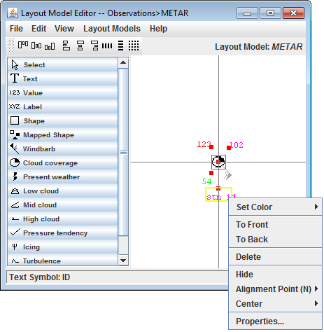
You can create your own station model from scratch by utilizing the File->New menu option, or you can select an existing station model with the Layout Models menu. The display includes a horizontal and vertical line, which acts as a reference point for the location of your station model with respect to the physical location of the observation (at the origin). The different shapes and features that you can add to the station model are in the left panel. They can be added to the station model by left-clicking the item and then clicking where you want to place it. Once in the Layout Model, individual components can be moved by left-clicking and dragging them. When you place an item into the station model, the Properties dialog for the component will open. You can also double click on an item to bring up its Properties dialog.
Each component of the station model can be resized by dragging the black squares along the outside of the item. You can select multiple items to align at once by holding down Shift and clicking on the items you wish to move. Each item in the station model also includes a red "Alignment Point', which acts to locate the individual components of the model with respect to the center point of the observation. The location of the Alignment Point to the item can be changed via the Alignment Point option in the menu when you right click on the item.
When you hold your mouse over a component of the station model, the name of the item will be listed in the bottom bar of the Layout Model Editor. This can be useful if you have multiple Value fields for text (temperature, dew point, etc.).
To save a station model you have composed, use the File->Save or File->Save As... menu items. When you save a station model, any point data displays that are using it will be updated. To remove a model, use the File->Remove menu item. You cannot remove a model supplied with McIDAS-V, but you can remove local models.
There are many options that you can control for each individual component of the station model. This menu is seen by right-clicking on an item.
The Properties window consists of four tabs: Display, Color By, Scale Size, and Rotate.
The Display tab allows you to assign which observation variable is associated with that item. Numerical values should appear in a "Value" item, text in a "Text" item, etc. Note that the items in this tab may differ depending on what item's properties you are displaying.
The Color By tab consists of two tabs within itself: Map Value Into Color Table, and Color From Parameter. This tab allows you to determine how you want to color your station model.
The Map Value Into Color Table tab allows you to color the parameter based off of its numerical value in relation to the set data range and color table for the parameter.
For example, in the above image the Temperature parameter has been specified with data range -90 to 45 Celsius. For each display, McIDAS-V will find the Temperature value (e.g., 15 Celsius), convert it to the specified unit (if necessary), find where it lays within the range, and use the corresponding color from the color table to display the data in the Main Display window.
The Color From Parameter tab allows you to specify parameter, a set of (regular expression) patterns, and a corresponding color. If the text value of the parameter matches one of the patterns then the given color is used to color the shape.
The Scale Size tab allows you to specify a parameter to scale the shape by. For each point display, McIDAS-V will find the value of the parameter, determine where that value lies within the data range, and find the corresponding scaling from the scale factor range.
The Rotate About Axis tab works like the scale and color by facilities. Note that the rotation is about the Z axis in X/Y/Z space. It is not a rotation in Lat/Lon space. All three tabs in the Rotate tab have the same fields.
Many of the menu items seen utilizing this display are standard options that can be found in the Menus section of the Layer Controls page. However, there are several options unique to this display.
The File menu has these unique options:
The Edit menu has these unique options:
The View menu has these unique options:
The Layout Models menu has these unique options:
The Parameter Alias Editor is opened through the Tools menu in the Main Display window with Tools->Parameters->Aliases menu and allows for the association between "canonical" parameter names used by McIDAS-V for physical quantities, such as TEMP for temperature, and parameter names used in particular data sets for the same quantity, such as for example "jan_mean_temp."
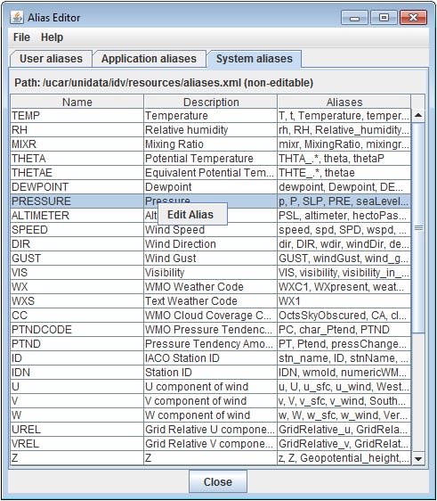
Different data sets often have different names for the same physical quantity, such as the quantities for temperature or easterly wind speed component. You can make McIDAS-V recognize any particular data name as representing a standard quantity. The Alias Editor associates any particular variable name that may appear in a data set (right column) with a canonical or McIDAS-V name or alias (left column).
The Alias Editor has a number of tabs that display the user editable aliases and the non-editable system aliases. You can right-click on a row in the System Alias tab to copy that row to the User aliases tab. You can edit a user's entry by right-clicking on the table row.
When you attempt to create a new alias, a Data Alias dialog is shown where you can edit the name, label (descriptive text) and the aliases:
The File menu has these unique items:
The Parameter Defaults Editor is opened through the Tools menu in the Main Display window with Tools->Parameters->Defaults and allows for the specification of default color tables, ranges, units, and contouring values for different parameters:
This feature lets you preset conventional color and contouring choices, and lets you override system defaults.
There are three sets of defaults: User defaults, Application defaults, and System defaults. While the items in the Application defaults and System defaults tabs cannot be modified within the tab, you can create a duplicate of the same parameter in the User defaults tab. If the same parameter is defined as a User default and an Application/System default, the User default will be used first. If you wish to modify an existing default, you can right-click on the item and select Copy Row to Users Defaults. When you do this the Parameter Defaults window allows you to select what properties you want to modify and define:
In the example above, any time a parameter named "rh" is used to define a field, the data will display with the Relative Humidity color bar, a range of 0-100, units of "%", and contour values as specified in the window. If you wish to define an individual item, such as Range, make sure the Defined checkbox is selected. If it is not checked, then any values stored in this window will not be saved as a default. From the User defaults tab, you can also right-click on a row to add a new row, edit the settings for the row, delete the row, or export an individual row as a plugin.
The parameter names are given in regular expression syntax to help match with actual data names. Plain text is matched exactly. The string dot star, ".*", means "any text here." The ^ means "begin with the following text exactly".
The File menu has these unique items:
The Parameter Groups Editor is opened through the Tools menu in the Main Display window with Tools->Parameters->Groups and allows for the specification of "parameter groups", named groups of parameter names.
There are two sets of defaults: user defaults in the tab User Groups, and system groups supplied with McIDAS-V in the System Groups tab. Look at the system defaults for examples.
The system settings cannot be edited by the user, but right clicking a row allows you to copy a group to the "user defined" table. When you do this the Parameter Groups Properties window allows you to define the sets of parameters that fall under this group.
The File menu has these unique items:
The Projection Manager allows you to choose, edit, and save map projections for use in McIDAS-V.
A projection is a way of mapping the surface of the Earth (a curved 2D surface) onto a flat 2D surface (a plane). A projection transforms a point on the earth (specified by latitude, longitude) to a point on the projection plane.
In the Projection Manager, both the projection and the area of the Earth can be specified. For example, you can make a Lambert Conformal map of North America, and a Lambert Conformal map of Sedgwick County, Kansas. Same projection, different areas.
McIDAS-V provides several basic types of projections: Lat/Lon, Lambert conformal conic, Transverse mercator, Stereographic, Mercator, Albers Equal Area, Lambert Azimuth Equal Area, Orthographic, VerticalPerspectiveView. Each of these can be parameterized (e.g., tangent point, origin longitude) to create a specific projection area of that type. When you define a projection and area, you specify the type of projection and its parameters.
You can bring up the Projection Manager with the Projections-> ![]() New/Edit... menu item in the Main Display window, or through the Tools->Projections->Edit Map Projections menu option in the Main Display window. Projections supplied with McIDAS-V are shown in the list. There may be additional projections you have created and named. In the figure, the US->CONUS projection is highlighted, and displayed on the left.
New/Edit... menu item in the Main Display window, or through the Tools->Projections->Edit Map Projections menu option in the Main Display window. Projections supplied with McIDAS-V are shown in the list. There may be additional projections you have created and named. In the figure, the US->CONUS projection is highlighted, and displayed on the left.
McIDAS-V starts with a default projection. Use the Default pulldown menu to select the projection that will be shown each time your McIDAS-V starts. (The default projection may not be used if you are starting McIDAS-V with a Bundle of configuration information).
This allows you to define new projections and to modify existing ones. Remember that a projection not only consists of the mathematical projection, but also the area of the Earth that is seen.
Here is how to create a new or revised projection:
Note that some fields in this window may be different depending on the map type you select. There are no Projection Parameters when using a Lat/Lon map type. In the example shown, a Lambert conformal conic projection is being defined with the projection parameters as shown in the figure.
McIDAS-V provides techniques to make computations with data sources and to display the results. The simplest technique is using McIDAS-V formulas, which are one-line mathematical expressions. The steps for computing and displaying the output of a McIDAS-V formula are:
Once you define a McIDAS-V formula, it is saved and will appear in future sessions of McIDAS-V.
To create a formula, select the Tools->Formulas->Create Formula menu item in the Main Display window. This opens the Formula Editor dialog window used to define a formula:
The formula itself can use common mathematical operators much as +, -, * for multiply, / for divide, and ** for power. Other Jython operations such as sqrt(a), max(b), pow(a,b), and sin(c) are available. The Jython Methods section of the User's Guide explains how to write complete multi-line functions or Jython methods that you can call in one-line formulas.
The variable names in the formula definition, such as "NIR" in the figure above, are operands and do not need to exactly match any particular parameter name in any data source; the association is made later, in the parameter selection step.
Do not use spaces in formula variable names, such as "wind speed." The formula is an expression in the Jython language. Each variable name must start with a letter.
It is best to use variable names that suggest the parameter data they represent, so that later you can easily remember what the variables mean. Use names like Temp500m, RelHum_surf, absvort, sst_jan, density, or whatever makes sense to you. If you use a variable names like V1 and V2, then later when the formula requests which real parameter name goes with which variable name you may be puzzled which is which.
Variable names can have extra "syntactic sugar" attached to them that McIDAS-V uses for a variety of purposes. The "sugar" consists of a set of name/value pairs contained in brackets ("[...]") after the variable name.
For example, normally variables are used to select and define data choices. You can also have variables that are simple text input from a user. For example, evaluating the following expression:
someProcedure(someValue[isuser=true])
will result in a dialog box being shown to allow for the user to enter a text value (e.g., a number) for the variable someValue.
You can provide default values with:
someProcedure(someValue[isuser=true,default=some default])
You can specify the types of data that can be selected for a variable with the categories name. e.g.:
someProcedure(someDataValue[categories=param:ALTITUDE])
If you want multiple data categories, separate them with a ";":
someProcedure(someDataValue[categories=param:ALTITUDE;param:elevation])
If you only want to select 3D grids do:
someProcedure(someDataValue[categories=GRID-3D-*])
If you only want to select 3D or 2D grids do:
someProcedure(someDataValue[categories=GRID-3D-*;GRID-2D-*"])
You can also specify a regular expression pattern that is used to pre-select the first data choice whose description matches the pattern.
someProcedure(someValue[pattern=some_pattern])
In the advanced section you can enter a description of the formula, its group or category, and you can define what types of displays are applicable for the given formula (the default is to be able to use all displays).
The group is used to display the formula in the Field Selector window and can be any alphanumeric text including spaces, numbers, and punctuation characters. Hyphens ("-") define sub-categories.
To save the formula, click on ![]() . A new entry appears in the selector panel. By right clicking on the formula entry in the Field Selector window you can edit the formula. If you edit a native formula and save it, the original formula will still be listed, but the modified formula will also be listed. To remove a formula, click on
. A new entry appears in the selector panel. By right clicking on the formula entry in the Field Selector window you can edit the formula. If you edit a native formula and save it, the original formula will still be listed, but the modified formula will also be listed. To remove a formula, click on ![]() in the pull down menu. You can also right click on a formula and select Remove Formula.
in the pull down menu. You can also right click on a formula and select Remove Formula.
For information about the Derived tab, see Derived Data.
McIDAS-V hides much of the computational complexity. You can write a simple formula such as (CT*1.8 + 32.0) - dewptF, and McIDAS-V will automatically apply the calculation to every element in large 3D grids referred to as CT and dewptF. No loops over grid points are needed; and you don't need to know anything about how the grid is defined, mapped on the Earth, or the data format. You can even use different sources for the individual parameters. For example, CT can come from a NAM model output grid and dewptF from your own local weather model. The two grids don't need to have the same grid point locations nor the same areal coverage. The results are computed in the area of overlap on the grid points locations of the first grid. Interpolation is automatically applied where needed.
Using a formula as the data when creating a display is just like using any other data. You select the formula entry in the Field Selector window, and the list of applicable displays will be shown and you create the display.
When you create a display, McIDAS-V needs to know what actual data should be bound to the operands within your formula. A Field Selector window will appear that allows you to select the actual data for each operand. You can select parameters from more than one data source for use in a single formula, for example, you can pick the same parameter from data sources of different times to compute a time difference in the parameter.
Open the data source to see the names of parameters available. Click on the parameter
needed for each variable. Then click ![]() . The result of the
formula is computed for every data point in the source, and the result shown
in the Main Display window.
. The result of the
formula is computed for every data point in the source, and the result shown
in the Main Display window.
As another convenience you can also right-click on the Formula: field of the Formula Editor to show the Insert Procedure Call menu. This lists all of the currently defined procedures in the other Jython libraries.
The Jython shell consists of an output window on the top and an input field
on the bottom. The user enters Jython into the input field. When Enter or ![]() is
pressed the Jython is evaluated and any output is shown in the output window. Note that Enter will only evaluate the field if the field has not been expanded. If your are using multi-line input for your commands, you can evaluate the commands with Shift+Enter.
is
pressed the Jython is evaluated and any output is shown in the output window. Note that Enter will only evaluate the field if the field has not been expanded. If your are using multi-line input for your commands, you can evaluate the commands with Shift+Enter.
The icons shown with every Jython entry in the output window allow you to select the particular Jython or re-evaluate it.
The entry window can be expanded with the ![]() to the right of the command line. When the entry field is expanded, you can enter more than one line of code to be processed at once. When the entry field isn't expanded, you are limited to evaluating one line of code at a time. As an alternative to the
to the right of the command line. When the entry field is expanded, you can enter more than one line of code to be processed at once. When the entry field isn't expanded, you are limited to evaluating one line of code at a time. As an alternative to the ![]() button, you can use Ctrl+/ to change between single and multi-line command line structure.
button, you can use Ctrl+/ to change between single and multi-line command line structure.
Pressing the "Up" arrow and "Down" arrow in the entry field goes up and down through the history of commands when you are in single-line input. If you are using multi-line input, use Ctrl+P, Ctrl+N to cycle through previously-executed commands.
After you have entered a and evaluated command, the command will be listed above the Evaluate field. To the right of the command, there are two buttons. The ![]() button enters the formula back into the Evaluate field without evaluating it. The
button enters the formula back into the Evaluate field without evaluating it. The ![]() button reevaluates the previously entered command without having to manually reenter it.
button reevaluates the previously entered command without having to manually reenter it.
Right-clicking in the entry field brings up a menu that allows you to:
All of the menu items in this tool are unique to the Jython Shell.
The File menu has these unique items:
The Edit menu has these unique items:
Apply the function name to each timestep of the data
applyToRangeValues(function, data):
Apply the function name to each value in each timestep of the data
averageOverTime(field, makeTimes):
Average the values in each time step If makeTimes is true (1) then we return a field mapping all of the times to the average. Else we just return the average
combine several fields together
extractLatitudeFromNWPGrid(fieldimpl):
Get the latitude coordinate from a grid. Return a grid of the latitudes at each point.
extractPressureFromNWPGrid(fieldimpl):
Get the pressure coordinate from a time series grid and return a grid of the pressure at all points. Input grid must have pressure or height (which is converted to pressure in the standard atmosphere). User must be sure input is a suitable FlatField.
Change units from geopotential meters to meters
getNthTimeGrid(fieldimpl, Nth):
Get the Nth grid in time series of grids; User must be sure input is a suitable data field. returns a single time. Nth is an integer, >=0, <= max index of grid time series.
getSliceAtAltitude(fieldimpl, alt, unit):
Extract a 2D horizontal slice from a 3D grid at the given altitude; level is a real number; if unit is supplied, it must be compatible with meters (ft, fathoms, etc) param fieldimpl is a grid which may have one or more time steps.
getSliceAtLevel(fieldimpl, level):
Extract a 2D horizontal slice from a 3D grid at "Level." level is a real number; must be appropriate for the grid. param fieldimpl is a grid which may have one or more time steps.
horizontalAdvection(param, u, v):
horizontal advection
horizontalDivergence(param, u, v):
horizontal flux divergence
layerAverage(grid, top, bottom):
Wrapper for calculating layer average
Wrapper for calculating layer difference
Make a 2D slice from a 3D slice at a single level
Make a vector from 3 components
makeVector(a,b) = [a,b,c]
Merge a set of single time grids/images into a time sequence
true wind vectors
Make a vector from 2 components
makeVector(a,b) = [a,b]
newName(field, varname, copy):
create a new field with a new parameter name
newUnit(field, varname, unitname):
set the name and unit on a grid
resampleGrid(oldGrid, gridwithNewDomain):
display gridded data on a new domain
windShear(u, v, z, top, bottom):
calculate the wind shear between discrete layers
shear = sqrt((u(top)-u(bottom))^2 + (v(top)-v(bottom))^2)/zdiff
windShearVector(u, v, top, bottom):
calculate the u and v layer difference and return as vector
writeGridToXls(grid, filename):
Write out the grid data to an excel spreadsheet
In the following operators, scalar operands are named Si and vector operands are named Vi. Lowercase u and v refer to the grid relative components of a vector.
Gravity constant
Addition
Horizontal Advection, negative by convention
Ageostrophic wind
Wrapper for atan2 built-in
Average of 2 scalars
Absolute Vorticity
Coriolis Parameter for all points in a grid
Vector cross product magnitude
Take the derivative with respect to the domain's X coordinate
Take the derivative with respect to the domain's Y coordinate
Total deformation
Horizontal Divergence
Vector dot product
Partial x derivative of a vector
Partial x derivative of a vector
Frontogenesis function from theta and the wind
geostrophic wind from height
Gradient of a scalar
Inertial advective wind
Jacobian Determinant
Laplacian operator
Latitudue all points in a grid
Layer Average
Layer Average
Magnitude of a vector
Mixing Ratio from Temperature, RH (requires pressure domain)
Multiply
Divide
Q-vector at a level ( K / m / s )
Horizontal Flux Divergence
Shear Deformation
Stretching Deformation
Subtract
Thermal wind
Potential Temperature from Temperature (requires pressure domain)
Equivalent Potential Temperature from Temperature and Relative humidity (requires pressure domain)
North relative u component
Grid relative u component
add the components of 2 vectors
Make a vector from two components
calculate the vector layer average
calculate the vector layer difference
Multiply the components of 2 vectors
North relative v component
Relative Vorticity
Divide the components of 2 vectors
Grid relative v component
subtract the components of 2 vectors
Magnitude of the vertical wind shear in a layer
combine 3 images as an RGB image
makeNavigatedImage(d, ulLat, ulLon, lrLat, lrLon):
This takes a image data object and a lat/lon bounding box and adds a lat/lon domain to the data. Use it in conjunction with a formula:
averageFromMap(field, mapSets):
mapSets defines a set of polygons. This procedure fills the areas in the field are enclosed by each polygon with the average value within that area
averageRangeFromMap(range, timeStep, mapSets):
mapSets defines a set of polygons. This procedure fills the areas in the field are enclosed by each polygon with the average value within that area
filterMaps(mapSets, propName, operator, value):
Return a new set of maps whose property propName satisfies the given operator/value. The operators can be ==,!=, <,>,<=,>=, match, !match
getMapProperty(polygon, propName):
Get the named property from the given mapData
getMapsWithProperty(mapSets, propName, value):
Return a new set of maps that have the given property value
Make a 3d map. map - map line data - topo - topography dataset
makeFieldFromMapBounds(mapSets, length1, length2, fill, unit):
Make a field whose lat/lon area is the bounds of the given mapSet. It has length1 points in the x and length2 in the y. Fill it with the fill value and the given unit
subsetFromMap(field, mapSets, fillValue, inverse):
mapSets defines a set of polygons. This procedure fills the areas in the field that are not enclosed by the polygons with the fill value. If inverse is 1 then it fills the areas that are enclosed
subsetRangeFromMap(range, timeStep, mapSets, fillValue, inverse):
mapSets defines a set of polygons. This procedure fills the areas in the field that are not enclosed by the polygons with the fill value. If inverse is 1 then it fills the areas that are enclosed
subsetRangeWithProperty(range, mapSets):
test code
subsetWithProperty(field, mapSets):
test code
Clear the shell
createDisplay(displayType, data, dataName):
create a display of type displayType. Right click in input field to select particular displayType. The data is can be a data object, a datachoice or a list of data or datachoices The dataName is used to name the data, i.e., its the parameter name
Find the data source object with the given name. If no name is given then this will return the first (non-formula) data source
getData(dataSourceName, dataChoiceName):
Find the data source with the given name and the data choice on that data source with the given name. If no dataSourceName is given then use the first one in the list If no dataChoiceName is given then use the first one held by the data source Return the data for the data choice. If no data source or data choice is found then return null
getDataChoice(dataSourceName, dataChoiceName):
Find the data source with the given name and the data choice on that data source with the given name. If no dataSourceName is given then use the first one in the list If no dataChoiceName is given then use the first one held by the data source Return the data choice If no data source or data choice is found then return null
List all of the variables defined in the shell's interpreter
Create a datasource from the given file name or url. The optional type parameter is used to specify the type of data
Print out the math type of the given data
selectData(name1, name2, name3, name4, name5):
Select up to 5 data fields. This returns a List of the actual Data objects
selectDataChoice(name1, name2, name3, name4, name5):
Select up to 5 data choices. This returns a List of the data choices, not the actual Data To get the data do:
The given dataSource can be an actual data source or the name of a data source. This procedure will define a set of jython variables that correspond to the data choices held by the given data source.
This procedure will define a set of jython variables, 'dataSource0, dataSource1, ...' that correspond to loaded data sources.
Bring up the jython library dialog
evaluate a formula
makeFloatArray(rows, cols, value):
A utility to make a 2 dimensional float array filled with the given value
The Display Settings facility allows you to select a set of properties from a display control (e.g., color table, contouring info, isosurface value, label template, etc.) and apply them to other display controls and/or save them as preferences to be used when creating new display controls.
The Display Settings dialog can be opened with the Edit->Display Settings... menu in the Layer Controls tab of the Data Explorer.
The left panel in this window is titled Source and includes two tabs, Displays and Saved Settings. The Displays tab includes all of the display types currently loaded into McIDAS-V. This tab is useful to make display settings changes within a session. If you wish, you can save these settings to be used in future sessions by using the File->Save Selected Properties menu item. The Saved Settings tab includes a list of any saved display settings you have made in previous sessions. You can store several different saved settings at once by grouping them into different categories.
The center panel of the window is titled Properties. These are the properties of the currently selected display control, which is shown highlighted in blue in the Source panel. On the right is also a list of target display controls.
The purpose of this is that you can select properties in the Properties panel that you want
to apply to the selected target display controls (via the checkboxes) on the
right. Many of the properties can be changed by clicking on the  buttons.
The View menu is useful for selecting different groups of target display controls. For example, you can select All Displays, displays of certain types, displays that have the same data sources, etc.
If you have two different data sources loaded with several displays created from each, normally the legend will list all of the displays based on some display category (e.g., Plan Views). However, you can change their display category so that each group of displays that are from one data source have the same category (e.g., "Data source 1", "Data source 2"). You can do this by changing the "Display Category" property under "Labels" to "Data Source 1".
Then, you could manually select the displays you want to change, or use the Select menu and choose "Displays with data source: ...":
This selects the displays with the data source of the currently selected display.
Once selected, you then hit ![]() , and the "Display
Category" will be set on the selected display controls.
, and the "Display
Category" will be set on the selected display controls.
To do the next set of displays, select a new Source display control in the list on the left. This will select this display and reset the properties list in the middle. Then, when you click Select->Displays with data source, the displays that share the data source from this new display will be selected.
You can save the set of selected settings with the File->Save Selected Properties option. The Save Display Settings dialog will be shown:
You can enter a category and a name. The saved settings will be shown under the Saved Settings tab. When selected they will be applied to the list of properties on the left. If you select the checkbox for Applicable only to displays of type, only the display listed will be an option in the Displays panel of the Field Selector.
The set of saved display settings are also shown in the Field Selector:
You can select any number of these, and when a new display control is created, these settings will be applied to the new display. The Show All checkbox allows you to list all of the settings, regardless if they were saved for a particular type of display.
Many of the menu items seen utilizing this display are standard options that can be found in the Menus section of the Layer Controls page. However, there are several options unique to this display.
The File menu has this unique option:
The Select menu has these unique options:
The Plugin Creator, accessed through the Tools->Plugins->Create... menu item in the Main Display window, allows you to create new plugins. The Plugin Creator is broken up into three tabs: Resources, Excludes, and Properties.
A plugin is a Java JAR file that contains a set of resource files. These resource files can include things like the color tables you have created, projections, station models, formulas, etc. The plugin manager supports both adding in a whole file (e.g., all of the color tables you have created) as well as adding in individual resource objects (e.g., a specific color table you have created).
To add in a file, use the File->Add File menu item. The file dialog will come up listing the contents of your local McIDAS-V directory. This is where all of the various resources that are created are stored. For example, if to include all of the color tables, add the colortables.xml file. Use the File->Add Preferences menu item to add your User Preferences to a resource, such as a bundle you are creating or editing. Individual resources can be added through the File->Add Resource menu item. Resources can also be added through the various resource editors (e.g., Jython Editor, Parameter Defaults, Parameter Aliases). Typically this facility is available through the editor's File menu.
Each file, preference, and resource that is added into the Plugin Creator is listed under the Resources tab:
Resources can be deleted by clicking the ![]() button or by pressing the delete key when a resource is selected.
button or by pressing the delete key when a resource is selected.
The Excludes tab allows for the exclusion of system default resources. For example, in the below image, Color tables and Map projections are excluded. When the plugin that is defined here is loaded into McIDAS-V, the excludes will result in only the Color tables and Map projections that are defined in this plugin to be used.
The Properties tab allows the user to overwrite different properties McIDAS-V uses. This listing is broken up into three categories: User Interface, Data, and Miscellaneous.
The User Interface category primarily affects the aesthetic appearance and basic usability in McIDAS-V. These options allow you to decide if you want to do the following:
The Data category affects what sources of data you will have available when selecting data in the Data Sources tab of the Data Explorer. These options allow you to decide the following:
The Miscellaneous category affects many features of McIDAS-V. While these options affect many things that go on 'under the hood' of McIDAS-V, there is a great deal that can be changed with these options. These options allow you to decide the following:
To write the plugin, click the ![]() button. If you have not specified a plugin file name, (i.e., a .jar file) you will be prompted. If you also want to install the plugin to your local McIDAS-V plugins area, select the Install checkbox. You can choose a specific location to save the plugin to by selecting the
button. If you have not specified a plugin file name, (i.e., a .jar file) you will be prompted. If you also want to install the plugin to your local McIDAS-V plugins area, select the Install checkbox. You can choose a specific location to save the plugin to by selecting the ![]() button, or by typing the file path into the field. Note: You will need to restart McIDAS-V for any installed plugins to take effect.
button, or by typing the file path into the field. Note: You will need to restart McIDAS-V for any installed plugins to take effect.
Many of the menu items seen utilizing the Plugin Creator tool are unique to this menu item.
The File menu has these unique options:
McIDAS-V plugins are a way to add to or modify the functionality of McIDAS-V. Plugins can range from adding new resources (e.g., color tables, layout models, maps) to changing the entire application. Plugins are typically Java JAR archive files that can contain a set of McIDAS-V resources and Java code. They are kept in a special directory on disk and are loaded at run time.
You can load a plugin (one time only) with the:
-plugin <plugin file or URL>
command line argument.
You can install a plugin with the:
-installplugin <plugin file or URL>
command line argument.
You can start McIDAS-V without any plugins with the:
-noplugins
command line argument.
The Plugin Manager, accessed through the Tools->Plugins->Manage... menu item in the Main Display window, allows you to list, install, and manage plugins.
A list of the installed plugins is shown at the top of the Plugin Manager, and a list of available plugins is shown below that. Click on an icon to perform an action in the Plugin Manager:
There are a few menu items that are unique to this tool.
The File menu has these unique options:
The Help menu has this unique option:
Bundles let you save a quick "snapshot" of McIDAS-V, including data sources, maps, and data displays. Bundles are small information files that specify the state of McIDAS-V. They are a kind of configuration file. They include information about what data sources are in use, and which parameters from the data sources are displayed, and how they are displayed.
The purpose of bundles is for you to save a particular McIDAS-V setup and display. A bundle can be used for your own reference at a later time, or others using McIDAS-V can use bundles you made to see data the same way you did.
To make a new bundle file, select the File->Save Bundle menu item in the Main Display window. A pop-up window will let you set a new file location and name:
The customary McIDAS-V bundle filename extension is .mcv; if you do not enter a file extension, .mcv will be appended. When saving a .mcv file, no data is saved with the bundle, only references to the remote or local Data Sources are saved.
McIDAS-V does support a zipped data bundle format: .mcvz. This is a zip file that contains a regular bundle (.mcv) and a set of data files. When the user does a "Save Bundle" or "Save Favorite " and specifies a .mcvz file extension, McIDAS-V prompts the user to select the data sources that should be written into the zip file. When opening a .mcvz file, McIDAS-V needs to unzip the data files, so it prompts the user as to where to place the files - a temporary directory or a user selected directory (this is a preference as well).
Note: In order for bundle files to work, the data must be available in exactly the same way you made connection to it when you made the bundle file. Others who use your bundles must have access to the same file system or to the same remote or local data servers you use, so that file paths or URLs to the data are exactly the same.
The file dialog has a set of buttons to define how parts of your bundle is saved.
Favorite bundles are just normal bundles that are categorized and saved off in a particular location on disk and serve as a convenience to the user. This allows the user to organize their favorites by category and readily load them in. Favorite bundles are easily available through the Bundles menu and can also be displayed on the toolbar of the Main Display window.
A favorite bundle can be created through the File->Save Favorite... menu item in the Main Display window:
Define your favorite bundle by specifying a category in the Category field and a name in the Name field. Categories can be hierarchical; by using a ">" as a separator (e.g. Toolbar>sounding) the categories will appear as a tree structure in the Local Favorites Bundles Manager. The "Toolbar" category is a special category in the Favorite Bundles Manager. The bundles in the Toolbar category will also appear as links in the toolbar of your Main Display window.
The Local Favorite Bundles Manager, accessed through the Bundles->Manage... menu item in the Main Display window, allows you to reorganize the categories and favorites by drag-and-drop, or right click on a favorite or a category to delete it, export it, etc.:
Once a bundle has been saved as a favorite, it can be set as your default bundle that will load automatically when you start McIDAS-V. You can set a default bundle in the Advanced tab of the User Preferences window. Note that after saving a favorite bundle, you must restart McIDAS-V before the bundle will be visible in the User Preferences window.
Use the File->Open File menu item in the Main Display window to open a bundle. When loading in a new bundle you will be prompted whether the current displays and data should be removed. You can also start up McIDAS-V with a bundle file or URL in the command line.
For most remote data types, data can be copied from the server to the local disk using the "Make Remote Data Local" facility. The following ADDE types are supported: satellite, radar, point, sounding and forecast fronts. There is also preliminary support for grids on remote servers* (see below).
This is used in two ways. First, the user can right-click on a data source in the Field Selector and select "Make Data Local" for remote data sources. McIDAS-V prompts for a file directory and a file prefix (the default is to use the name of the data source) and the remote data is copied over. For multiple files the format used is: <directory><prefix><file count>.<suffix>. The data source object within McIDAS-V is then changed to point to the new file paths.
The second way this is used is when a .mcvz file is saved. The user is prompted for both the local data sources to be saved off as well as for the remote data sources. For the remote ones, McIDAS-V automatically copies the files over and zips them.
*Grids: There is preliminary support for grids. This support relies on some extra service information in the catalogs which, right at this moment, is not included in the regular IDV gridded data catalog but is included for model data under the "File_Access" dataset in the main thredds catalog: http://www.unidata.ucar.edu/georesources/threddsRtModels.xml When saving gridded data the user is prompted for the fields to save and the geo-spatial subset is used to subset the grids. As of right now, there is not yet support for sub-setting on times and grid stride/decimation.
McIDAS-V has the ability to load and save IDV bundles (.xidv and .zidv), but all of the features between the two software packages may not be compatible, and therefore the bundles may not load properly in the other software package.
McIDAS-V can be scripted to create and manipulate images and movies. The scripting is accomplished using Jython. Jython is an implementation of the Python language in Java and follows Python syntax.
McIDAS-V scripting can be done from the Jython shell, or a Jython script can be invoked as a command line argument.
In Unix, from the McIDAS-V-System directory:
runMcV -script /home/user/example.pyIn Windows, from the McIDAS-V System directory (if running under a Windows machine, it is necessary to use "\\" instead of "\" in scripts when specifying directory paths to avoid Windows interpreting it as an escape sequence.):
runMcV.bat -script C:\\home\\user\\example.py
When invoked as a command line argument, the user interface will not be shown. However, McIDAS-V still needs to be run with an active window system (e.g., X, MS Windows) for it to run. If running under a Linux/Unix machine with no X server running, McIDAS-V must be run under the X virtual frame buffer, xvfb.
McIDAS-V supports a number of functions and methods to load and display data, manipulate the display, and to save images. Download the example script to see how to use each one (example.py). This page contains a list of funtions that are supported in McIDAS-V. You can find more information about each function, including parameters, keywords, and example commands, by clicking on a function or a function category.
For users looking for more functionality from McIDAS-V scripting, additional functions can be found in the Java docs for visAD, netCDF, IDV, and McIDAS-V. Please send any questions or requests for functionality to the McIDAS-V Support Forum on scripting.
buildWindow - Creates a window and returns an array of panels (single panel currently supported)
| height= | height of the window |
| width= | width of the window |
| panelTypes= | type of display to create MAP (default) GLOBE |
openBundle - Creates a new window and displays contents of a bundle
| height= | height of display; default= height of the display window when the bundle was saved |
| width= | width of display; default= width of the display window when the bundle was saved |
| dataDirectory= | a dictionary where the keys are datasource names, and the values are either a string or list of strings representing the full path name/names of the data that will be used in place of the data in the bundle |
| mode= | specifies the method that will be used to open the bundle REPLACE - Removes any previously-loaded layers and data sources and replaces the current session with the bundle's data (default) NEWWINDOW - Loads the bundle's data and displays into a new window, without removing any previously-loaded layers and data sources MERGE - Loads the bundle's data and displays into the current tab of the active display window without removing any previously-loaded layers and data sources NEWTAB - Loads the bundle's data and displays into a new tab of the active display window without removing any previously-loaded layers and data sources |
makeLocalADDEEntry - Creates a local ADDE entry in the server table
| dataset= | name of the dataset - limit of 8 characters |
| imageType= | image type name for local server entry. (default=format_dataset) |
| save= | True - saves entry into the server table; False - entry is removed after McIDAS-V session is ended (default) |
| mask= | directory containing the files used by the created dataset |
| format= | data format of files within the dataset. Either Full Name or Short Name can be used as valid options: |
| Full Name | Short Name |
|---|---|
| "AMSR-E L1b" | "AMSR" |
| "LRIT GOES-9" | "FSDX_G9" |
| "LRIT GOES-10" | "FSDX_G10" |
| "LRIT GOES-11" | "FSDX_G11" |
| "LRIT GOES-12" | "FSDX_G12" |
| "LRIT MET-5" | "FSDX_M5" |
| "LRIT MET-7" | "FSDX_M7" |
| "LRIT MTSAT-1R" | "FSDX_MT" |
| "McIDAS Area" | "AREA" |
| "Meteosat OpenMTP" | "OMTP" |
| "Metop AVHRR L 1b" | "LV1B_METOP" |
| "MODIS MOD 02 - Level 1B Calibrated Geolocated Radiances" | "MODS" |
| "MODIS MOD 04 - Aerosol Product" | "MOD4" |
| "MODIS MOD 06 - Cloud Product" | "MODX_06" |
| "MODIS MOD 07 - Atmospheric Profiles" | "MODX_07" |
| "MODIS MOD 28 - Sea Surface Temperature" | "MOD8" |
| "MODIS MOD 35 - Cloud Mask" | "MODX_35" |
| "MODIS MOD R - Corrected Reflectance" | "MODR" |
| "MSG HRIT FD" | "MSGT_FD" |
| "MSG HRIT HRV" | "MSGT_HRV" |
| "MTSAT HRIT" | "MTST" |
| "NOAA AVHRR L 1b" | "LV1B_NOAA" |
| "SSMI" | "SMIN" |
| "TRMM" | "TMIN" |
| "GINI" | "GINI" |
getLocalADDEEntry - Gets the descriptor for a local ADDE entry
| dataset= | local ADDE entry dataset name |
| imageType= | image type of local ADDE entry |
getADDEImage - Requests data from an ADDE Image server - returns both data and metadata objects
| localEntry= | local dataset defined by makeLocalADDEEntry |
| server= | ADDE server |
| dataset= | ADDE dataset group name |
| descriptor= | ADDE dataset descriptor |
| day= | single day ('date 1') or as a day range ('begin date','end date') |
| time= | ('begin time','end time') |
| coordinateSystem= | coordinate system to use for retrieving data AREA = AREA file coordinates - zero based LATLON = latitude and longitude coordinates IMAGE = image coordinates - one based |
| location= | (x,y) x = AREA line, latitude, or IMAGE line y = AREA element, longitude, or IMAGE element |
| place= | CENTER places specified location (x,y) at center of panel ULEFT places specified location (x,y) at upper-left coordinate of panel |
| band= | McIDAS band number; must be specified if requesting data from multi-banded image; default=band in image |
| unit= | calibration unit to request; default = 'BRIT' |
| position= | time relative (negative values) or absolute (positive values) position in the dataset; default=0 (most recent image) |
| size= | number of lines and elements to request; default=(480,640) |
| mag= | magnification of data (line,element), negative number used for sampling data; default=(1,1) |
| accounting= | ('user', 'project number') user and project number required by servers using McIDAS accounting; default = ('idv','0') |
| debug= | send debug information to file; default=False |
listADDEImages - Lists data from an ADDE Image server that matches the keywords in the request - returns metadata objects which can be passed into getADDEImage
| localEntry= | local dataset defined by makeLocalADDEEntry |
| server= | ADDE server |
| dataset= | ADDE dataset group name |
| descriptor= | ADDE dataset descriptor |
| day= | single day ('date 1') or as a day range ('begin date','end date') |
| time= | ('begin time','end time') |
| coordinateSystem= | coordinate system to use for retrieving data AREA = AREA file coordinates - zero based LATLON = latitude and longitude coordinates IMAGE = image coordinates - one based |
| location= | (x,y) x = AREA line, latitude, or IMAGE line y = AREA element, longitude, or IMAGE element |
| place= | CENTER places specified location (x,y) at center of panel ULEFT places specified location (x,y) at upper-left coordinate of panel |
| band= | McIDAS band number; must be specified if requesting data from multi-banded image; default=band in image |
| unit= | calibration unit to request; default = 'BRIT' |
| position= | time relative (negative values) or absolute (positive values) position in the dataset; default=0 (most recent image) |
| size= | number of lines and elements to request; default=(480,640) |
| mag= | magnification of data (line,element), negative number used for sampling data; default=(1,1) |
| accounting= | ('user', 'project number') user and project number required by servers using McIDAS accounting; default = ('idv','0') |
| debug= | send debug information to file; default=False |
listADDEImageTimes - Returns a list of available dates and times of data that match the keywords in the request
| localEntry= | local dataset defined by makeLocalADDEEntry |
| server= | ADDE server |
| dataset= | ADDE dataset group name |
| descriptor= | ADDE dataset descriptor |
| day= | single day ('date 1') or as a day range ('begin date','end date') |
| time= | ('begin time','end time') |
| coordinateSystem= | coordinate system to use for retrieving data AREA = AREA file coordinates - zero based LATLON = latitude and longitude coordinates IMAGE = image coordinates - one based |
| location= | (x,y) x = AREA line, latitude, or IMAGE line y = AREA element, longitude, or IMAGE element |
| place= | CENTER places specified location (x,y) at center of panel ULEFT places specified location (x,y) at upper-left coordinate of panel |
| band= | McIDAS band number; must be specified if requesting data from multi-banded image; default=band in image |
| unit= | calibration unit to request; default = 'BRIT' |
| position= | time relative (negative values) or absolute (positive values) position in the dataset; default=0 (most recent image) |
| size= | number of lines and elements to request; default=(480,640) |
| mag= | magnification of data (line,element), negative number used for sampling data; default=(1,1) |
| accounting= | ('user', 'project number') user and project number required by servers using McIDAS accounting; default = ('idv','0') |
| debug= | send debug information to file; default=False |
createLayer - Creates a new data layer in a panel
annotate - Writes text to a panel
| lat=, lon= | center text string at specified latitude and longitude (must be used together) |
| line=, element= | center text string at specified panel line and element (must be used together) |
| font= | name of font; default is system dependent, this uses the default defined in User Preferences |
| size= | size of font; default = size of font defined in user preferences |
| color= | 'color name'; default = 'red' -or- [R,G,B] fractional scaling factor for each red, green and blue value (0 to 1) |
setCenter - Centers the display on a specified latitude/longitude and sets a scaling factor
| scale= | scale factor for map; default = current scale factor |
setProjection - Sets the projection of a panel
setWireframe - Turns wire frame box on or off
| visible= | True - displays color scale (default) |
| placement= | location of color scale 'Top' (default) 'Bottom' 'Left' 'Right' |
| font= | name of font; default = font defined in User Preferences |
| style= | font style; default=font defined in user preferences 'BOLD' - bolded font 'ITALIC' - italicized font 'NONE' |
| size= | size of font; default = size of font defined in User Preferences |
| color= | 'color name'; default = color defined in User Preferences -or- [R,G,B] fractional scaling factor for each red, green and blue value (0 to 1) |
| showUnit= | toggles the visibility of the display unit on the color scale (default = False) |
setEnhancement - Applies
a color table and defines data range of data in a layer
| range= | (min,max) enhancement range; default = (min,max) of data |
setLayerLabel - Toggles a layer label on/off and defines its attributes
| visible= | True - displays layer label(default) |
| font= | name of font; default = font defined in User Preferences. |
| style= | font style; default = font defined in user preferences 'BOLD' - bolded font 'ITALIC' - italicized font 'NONE' |
| size= | size of font; default = size of font defined in User Preferences |
| color= | 'color name'; default = color defined in User Preferences -or- [R,G,B] fractional scaling factor for each red, green and blue value (0 to 1) |
setLayerVisible - Toggles layer visibility on/off
| height= | height of image (default - see Remarks) |
| width= | width of image (default - see Remarks) |
| quality= | quality of jpg file (0.0 to 1.0); default=1.0; not used with other formats |
writeMovie - Writes
an image sequence to a movie file (ISL function)
| resize width= height= | size of image (default = height of window) |
setJythonShellMaxHistoryLength( ) - Sets the number of commands that will be saved.
collectGarbage( ) - Performs a garbage collection to free up memory.
removeAllData( ) - Removes all data sources added during the current session, without removing any displays.
removeAllLayers( ) - Removes all layers that have been displayed.
expandpath( ) - Expands the path entered.
editFile( ) - Pastes the content of a text file into the text input field of the Jython Shell.
getLogLevel( ) - Sets the logging level to be used by McIDAS-V.
| level- | The logging level of the directory path used in the command. If a directory path is not specified, this is the logging level for the session as a whole. |
| effectiveLevel- | The logging level for the specific module specified in the command |
setLogLevel( ) - Sets the logging level to be used by McIDAS-V.
| temporary= | determines if the logging level will be saved from session to session (default = True) |
For sharing animation in two windows, such as in the main McIDAS-V view window and a vertical cross section control, open the animation properties dialog in each animation control by clicking on the ![]() icon. Toggle on the Shared box and click on Ok. Then using either animation control will effect animation in both windows.
icon. Toggle on the Shared box and click on Ok. Then using either animation control will effect animation in both windows.
You can share other kinds of layer controls, such as sharing one selector line in vertical cross sections. This is toggled on by clicking on the Share checkbox under the View menu in the control window.
By default McIDAS-V looks in three places for the resources it uses to configure itself:
idv.properties = %SITEPATH%/idv.properties;%USERPATH%/idv.properties;You can also specify one or more properties files as command line arguments:
-properties your_properties_fileMcIDAS-V processes these properties files in order, with properties defined in later files overriding those defined previously.
Once the properties have been processed McIDAS-V initializes its resources by reading in one or more resource definition files. These are called "RBI" files - (Resource Bundle for the IDV). These are XML files, the locations of which are defined by the idv.resourcefiles property:
idv.resourcefiles=%USERPATH%/idv.rbi;%SITEPATH%/idv.rbi;%IDVPATH%/idv.rbiWhen you first run McIDAS-V, the application writes out an example RBI file into your local McIDAS-V directory. This example file has documentation that describes how to add in new resources.
These RBI files define the location of different collections of resources. For example, from the system RBI file, idv.rbi, we have the entry that defines where McIDAS-V can find the XML files that define the color tables:
<resources name="TARGET_SiteConfiguration__idv.resource.colortables">
    <resource location="%USERPATH%/colortables.xml"/>

    <resource location="%SITEPATH%/colortables.xml"/>

    <resource location="%IDVPATH%/colortables.xml"/>

  </resources>
This says to look for colortables in the user path, sitepath and McIDAS-V system path. McIDAS-V uses the first entry in this list as the file path to write out color tables that are created using the color table editor.
Note: As a further, convenience, if there is a property defined in the properties file which is the resource name then McIDAS-V just uses the value of the property (it treats it as a semi-colon delimited list of paths) as the resources and ignores the resources in the RBI file. So, for example, if you had a property:
idv.resource.colortables=%USERPATH%/colortables.xml;http://yourwebsite.edu/specialtables.xmlthen McIDAS-V would only load in these colortables.
To use the RBI file, you need to configure your site to use a set of special color tables that you have created. The first thing to do is bring up McIDAS-V and create the color tables. These color tables get saved in your local McIDAS-V/<Application name> directory in the file colortables.xml (as defined by the resource paths defined in the default RBI). You could copy that file to an area on your web site or on a shared file system that is pointed to by the McIDAS-V sitepath. Now, your users simply need to define the sitepath and they will naturally pick up the color tables you have created.
Most site configuration can be accomplished through the default user/site/system resource locations. However, you can modify the RBI file to include other resources. For example, you could add in an entry:
<resource location="http://yourwebsite.edu/specialcolortables.xml"/>to make available some special color tables at a particular URL.
| Resource Identifier | Description | File Pattern |
| idv.resource.colortables | Color tables used in the application | colortables.xml$ |
| idv.resource.projections | Map projections | projections.xml$ |
| idv.resource.transects | Map transects | transects.xml$ |
| idv.resource.messages | Message catalog | messages.properties$ |
| idv.resource.grib1lookuptables | Grib 1 Lookup tables | grib1lookuptable.lst$ |
| idv.resource.grib2lookuptables | Grib 2 Lookup tables | grib2lookuptable.lst$ |
| idv.resource.jython | Jython libraries | .py$ |
| idv.resource.stationmodels | Station models | stationmodels.xml$ |
| idv.resource.imagedefaults | ADDE Image Defaults | imagedefaults.xml$ |
| idv.resource.backgroundwms | Background WMS images | backgroundwms.xml$ |
| idv.resource.imagesets | Image Sets | imagesets.xml$ |
| idv.resource.autodisplays | Automatic display creation | autodisplays.xml$ |
| idv.resource.skin | UI Skin | skin.xml$ |
| idv.resource.toolbar | Tool bar | toolbar.xml$ |
| idv.resource.actions | Actions | actions.xml$ |
| idv.resource.stationsymbols | Station model symbols | stationsymbols.xml$ |
| idv.resource.colorpairs | Color pairs | no pattern |
| idv.resource.bundlexml | Bundle xml | no pattern |
| idv.resource.aliases | Data aliases | aliases.xml$ |
| idv.resource.datasource | Specification of the data sources | datasource.xml$ |
| idv.resource.derived | Derived quantities | derived.xml$ |
| idv.resource.choosers | The definition of the user interface for data choosers | choosers.xml$ |
| idv.resource.bundles | Default bundles that are evaluated at start up | no pattern |
| idv.resource.controls | Display controls | controls.xml$ |
| idv.resource.helptips | Help tips shown in the help tips dialog | helptips.xml$ |
| idv.resource.locations | Fixed station locations | locations.xml$ |
| idv.resource.maps | Maps for the displays | maps.xml$ |
| idv.resource.menubar | Commands in the menu bar | (defaultmenu.xml$|menubar.xml$) |
| idv.resource.paramdefaults | Display defaults for data | paramdefaults.xml$ |
| idv.resource.paramgroups | Parameter groups | paramgroups.xml$ |
| idv.resource.userchooser | End user constructed data choosers | no pattern |
| idv.resource.preferences | User preferences | no pattern |
| idv.resource.plugins | Plugins | no pattern |
| idv.resource.prototypes | Prototypes | no pattern |
McIDAS-V supports a plugin architecture that allows for the easy extension and addition of functionality. A plugin is most commonly a Java Jar file that contains a set of resource files (e.g., color tables) and/or Java class files. The plugins are stored on a local directory or could be loaded form a web site. McIDAS-V processes the plugin Jar file at run time loading in the contained resources and code.
To make these into a plugin, e.g., myplugin.jar, simply jar the the files (you need to get a Java SDK for this):
jar -cvf myplugin.jar colortables.xml default.py
Now this plugin can be distributed to others and loaded into their McIDAS-V environment.
So, you might ask how does McIDAS-V recognize these files in the plugin and treat them appropriately? McIDAS-V loads in a set of resources (e.g., color tables, Python libraries). Each resource type is identified by a regular expression as shown in the resource list. In our example above the file name colortables.xml matches the pattern for color table xml resources.
Now, what happens if you have some file whose name does not match a pattern? Say, you have a color table xml file called myspecialtables.xml that you want to include in a bundle. In that case you can add a .rbi file, as described here, that defines this file as a resource:
<?xml version="1.0" encoding="ISO-8859-1"?>

<resourcebundle>

<resources name="TARGET_PluginJarFiles__idv.resource.colortables">
    <resource location="/myspecialtables.xml"/>

  </resources>

</resourcebundle>
This acts as a table of contents for the plugin. Make sure that the location
is not relative. Note: Jar files can contain directory trees. e.g., /tables/myspecialtables.xml.
In this case just have the location point to:
...

    <resource location="/tables/myspecialtables.xml"/>

...
/edu/ucar/app/Test.class
For a single class file this is not necessarily required but if there are multiple class files that have interdependency among themselves then you will get into trouble if you don't follow this structure.
Now, what this code does can be anything and is best left up to the developer's guide.
<?xml version="1.0" encoding="ISO-8859-1"?>

<imagedefaults>

  <default

     pattern=""

     key=""

     place=""

     loc=""

     unit=""

     user=""

     band=""

     proj=""/>

</imagedefaults>
The attributes that can be overridden are:
| pattern | dataset identifier (format: host:group/desc) |
| key | type of location (LINELE or LATLON) |
| place | placement (ULEFT or CENTER) |
| loc | location of placement (line ele or lat lon) |
| size | resulting image size (lines eles) |
| mag | magnification factor (lmag emag) |
| unit | default calibration unit |
| band | band number |
| proj | project number |
| user | user id (case sensitive) |
| debug | (true to print lots of debug information) |
Here are a few examples:
<imagedefaults>


    <default pattern="*" debug="true"/>


    <default

        pattern="adde.ucar.edu:RTIMAGES/GE-IR"

        key="LATLON"

        place="CENTER"

        loc="40 -90"

        unit="BRIT"

        user="foo"

        proj="9999"/>


    <default

        pattern="EUM_AD/M8"

        loc="46 10"

        band="9"

        unit="TEMP"

        size="512 512"/>


    <default

        pattern="CIMSS/CTP"

        key="LATLON"

        loc="35 -100"

        mag="1 1"

        unit="CTOP"/>


    <default

        pattern="GINICOMP/GSN8KVIS"

        key="LINELE"

        place="CENTER"

        loc="504 768"

        size="504 768"

        mag="-2 -2"/>


    <default

        pattern="CCS039/G81KVIS"

        key="LINELE"

        place="ULEFT"

        loc="0 0"

        size="ALL"/>


</imagedefaults>
McIDAS-V can read Gridded Binary (GRIB) files in both GRIB-1 and GRIB-2 formats. Decoding GRIB files requires a set of lookup tables for parameters, issuing centers, etc. McIDAS-V comes pre-configured to support commonly used tables, but regional models and modeling centers may use tables that are not in the distribution.
You can add in specialized tables for both GRIB-1 and GRIB-2 using the steps below. Documentation on the format of the files can be found here.
To add in new GRIB 1 tables, you will need to create a file listing the special tables and the special table files themselves.
To add in a new parameter file, McIDAS-V would need to have access to a file called grib1lookuptable.lst which would list the parameter table (e.g.: gwctab_2.tab) and the parameter table itself.
The format of grib1lookuptable.lst is:
<center>:<subcenter>:<version>: <table location>
so it would look like:
57: 1: 2: gwctab_2.tab
gwctab_2.tab can be a relative or absolute path. The tables are in ncep format:
-1:57:-1:2

0:var0:undefined

1:PRES:Pressure [Pa]

2:PRMSL:Pressure reduced to MSL [Pa]

3:PTEND:Pressure tendency [Pa/s]

4:PVORT:Pot. vorticity [km^2/kg/s]

5:ICAHT:ICAO Standard Atmosphere Reference Height [m]

:GP:Geopotential [m^2/s^2]

...
(You can read more information about the format of this file and the parameter table here)
Once you've created this file, you would access it by putting the grib1lookuptable.lst in your <home>/McIDAS-V directory and put the corresponding table files where they are pointed to in the file. This can be a relative path or a web server. Alternatively, you could place the grib1lookuptable.lst and associated parameter tables on a local web server and use McIDAS-V's sitepath parameter (startup option or user preference) to point to the location where the files are.
To add in new GRIB 2 parameter, you would create a file named grib2lookuptable.lst which lists the parameters.
The format of grib2lookuptable.lst is:
<Discipline> <Category> <Parm #> <Name> <Units> <Desc>
Parameters are listed by row, fields are separated by tabs, so it would look like:
#Dis    Cat     Parm #  Name            Units   Desc

0       0       0       Temperature     K       Temperature
(This is a sample table, the lines starting with # are not include in table.) (You can read more information about the format of this file and the parameter table here)
Once you've created this file, you would access it by putting the grib2lookuptable.lst in your <home>/McIDAS-V directory. Alternatively, you could place the grib2lookuptable.lst on a local web server and use McIDAS-V's sitepath parameter (startup option or user preference) to point to the location of the file.
You need to specify the metadata of this point data. This can be done in two ways. First, the file can have two extra header lines that defines for McIDAS-V the fields that are within the file and the types of the fields. The only other requirement is that there must be a latitude, longitude and time field in the data. See below.
Secondly, if there are no metadata header lines defined, the Text Point Data Source will show the Metadata GUI described below.
More information about the format of Time and Lat/Lon symbols can be found in the User Preferences' Formats and Data Preferences page.
(index) -> (Time,Latitude,Longitude,Altitude,PSL,GUS,SPD,DIR,TD,T)

Time[fmt="yyyy-MM-dd HH:mm:ss"],Latitude[unit="deg"],Longitude[unit="degrees west"],Altitude[unit="m"],PSL[unit="hPa"],GUS[unit="m.s-1"],SPD[unit="m/s"],DIR[unit="deg"],

TD[unit="celsius"],T[unit="celsius"]

2007-01-07 16:00:00Z,32.9,117.1,145.0,1026.1,NaN,0.0,0.0,-2.8,12.8

2007-01-07 16:00:00Z,48.3,92.5,341.0,1003.7,NaN,1.5,170.0,-2.0,-0.99

2007-01-07 16:00:00Z,36.8,98.7,449.0,1024.0,12.4,9.8,330.0,-3.0,3.0

2007-01-07 16:00:00Z,44.3,121.2,938.0,1030.1,NaN,2.1,110.0,-3.3,-1.7
Note also that the first line's structure is quite rigid -- you must have a variable (e.g., index, recNum) that is the domain parameter; this should map to the range values. The second line defines the formatting and units of the parameters. Unit names should be standard international unit specifications (udunits compatible). A list of valid names can be found here. (A complete description of this format is contained in the VisAD README.text file.)
Also note that you need to set the name of the variable for time as "Time", as well as the locations as "Latitude", "Longitude" and "Altitude" (if needed).
(index) -> (Time,Latitude,Longitude,Altitude,ST(Text),T)

Time[fmt="yyyy-MM-dd HH:mm:ss z"],Latitude[unit="deg"],Longitude[unit="degrees west"],Altitude[unit="m"],ST(Text),T[unit="celsius"]

2007-02-16 11:00:00 MST,32.9,117.1,145.0,CA  ,20.6
Here we have a ST field (State from metars). Its field name is defined as "ST(Text)" and its entry in the second line is the same.
(index) -> (IDN, Latitude, Longitude, Time, WDIR, WSPD, GST)

IDN, Latitude[unit="deg"], Longitude[unit="deg"], Time[fmt="yyyy MM dd HH mm" colspan="5"], WDIR[unit="deg" miss="MM"], WSPD[unit="m/s" miss="MM"], GST[unit="m/s" miss="MM"]

41001 34.68 -72.66 2007 07 17 20 50 210 4.0 6.0

41004 32.5 -79.09 2007 07 17 20 50 210 6.0 MM

41008 31.4 -80.87 2007 07 17 21 50 170 7.0 8.0
(recNum)->(Latitude, Longitude, Altitude, type(Text), time, turb_intensity)

time[fmt=yyyyMMddHH], obtime, skip, type(Text), skip, skip, Latitude, Longitude[scale=-1], Altitude[unit=ft], Altitude2[unit=ft], turb_intensity, skip

2004050100 0005    34     C210 1 T  38.82   92.22   7000   7000  0 -9

2004050100 0004    35     PA32 0 T  35.40   98.62   4000   4000  0 -9

2004050100 0008    58      A36 0 T  29.18   81.05   5000   5000  2 -9
(index) -> (Longitude,Latitude,Time,ST(Text),SPD,DIR,TD,T)

Longitude[unit="degrees west"],Latitude[unit="deg"],Time[fmt="yyyy-MM-dd HH:mm:ss z"],ST(Text),SPD[unit="m/s"],DIR[unit="deg"],TD[unit="celsius"],T[unit="celsius"]


Longitude=-117.1

Latitude=32.9

ST=MSN

2007-02-20 11:00:00 ST  ,0.0,0.0,8.9,13.3

2007-02-20 12:00:00 ST  ,0.0,0.0,11.9,15.0


Longitude=-89.4

Latitude=43.1

ST=DEN

2007-02-20 11:00:00 ST  ,1.5,160.0,-7.0,-2.0

2007-02-20 12:00:00 ST  ,1.5,160.0,-7.0,-2.0


Longitude=-121.2

Latitude=44.3

ST=ORD

2007-02-20 11:00:00 ST  ,10.8,230.0,-1.1,6.7
Delimiter
This field specifies how the different data values are separated within the text file. The options are Comma, Semicolon, Tab, and Space. Selecting this option allows McIDAS-V to separate out different text fields to allow you to define them at the bottom of this Point Data window.
Skipping lines
At the top, a number of the initial lines from the text data are shown. The arrow keys allow you to specify the start line. For example, if you had some other header information, you can skip over those lines.
Specifying metadata
For each column of text data there is a row shown in the bottom of the dialog. This shows the sampled value and allows you to enter a name, unit, date format, missing value and extra information. There are some names that McIDAS-V treats special: "Latitude", "Longitude", "Altitude", and "Time". You must have at least Latitude, Longitude and Time specified.
The Unit/Date Format field allows you to specify the Unit for data fields and the date format. For text fields choose Misc->Text as the unit.
The Extra fields must be of the form:
name="value"Don't forget the quotes!
Skipping columns
You can skip over certain columns by entering the Name: "skip"
Saving this as a preference
To keep from having to enter in this data again next time you load a new text point data of the same form, simply press the "Preferences" button and select Save
Current. This allows you to save these metadata settings and reapply them later
using the "Preferences" button.
McIDAS-V supports a variety of location text file formats. All of these formats can be loaded through the File Chooser. Select the "Location" data type.
The main one format McIDAS-V uses is a custom locations xml format. This format still has some nomenclature from when it was atmospheric science related (e.g. "stations"). A simple example:
<?xml version="1.0" encoding="ISO-8859-1"?>

<stationtable name="TARGET_LocationXml__Example">
<station name="TARGET_LocationXml__station 1"  lat="65:02:06" lon="-147:30:06" elev="790"/>
<station name="TARGET_LocationXml__station 2"  lat="40.3" lon="-107.5" elev="10"/>
    ...

</stationtable>
The lat and lon attributes can be of the form:
    +/-  ddd:mm, ddd:mm:, ddd:mm:ss, ddd::ss, ddd.fffff ===>   [+/-] ddd.fffff

    +/-  ddd, ddd:, ddd::                               ===>   [+/-] ddd

    +/-  :mm, :mm:, :mm:ss, ::ss, .fffff                ===>   [+/-] .fffff

    +/-  :, ::                                          ===>       0.0

    Any of the above with N,S,E,W appended
The elev attribute is optional. By default it is in meters. You can override this default with an elevunit in the stationtable tag. e.g.:
<?xml version="1.0" encoding="ISO-8859-1"?>

<stationtable name="TARGET_LocationXml__Example" elevunit="feet">
<station name="TARGET_LocationXml__station 1"  lat="65:02:06" lon="-147:30:06" elev="5340"/>
...
The station tags can have an id attribute as well:
<station  id="APD" name="TARGET_LocationXml__Fairbanks/Pedro Dome"
          lat="65:02:06" lon="-147:30:06" elev="790"/>
The station tags can also have any other attributes:
<station  id="APD" name="TARGET_LocationXml__Fairbanks/Pedro Dome"
          st="AK" co="US"

          lat="65:02:06" lon="-147:30:06" elev="790"/>

<station id="FTG" name="TARGET_LocationXml__Denver/Boulder"
         st="CO" co="US"

         lat="39:47:12" lon="-104:32:45" elev="1675"/>
These can be displayed by the station model used in the Location Display Control.
If you want to create a permanent list of station that shows up in the Display->Locations menu in the Main Display window, you can create a file called userstations.xml in the McIDAS-V directory under your user's home directory. The format would look like:
<?xml version="1.0" encoding="ISO-8859-1"?>

<stationtables>


<stationtable name="SubsetA" category="My Custom Stations">

(list of stations for SubsetA)

</stationtable>


<stationtable name="SubsetB" category="My Custom Stations">

(list of stations for SubsetB)

</stationtable>

</stationtables>
This will show up in the Display->Locations menu as a top menu called My Custom Stations and sub menus SubsetA and SubsetB. After adding this XML file in through the Files/Directories chooser, you must first restart McIDAS-V before the stations will be listed.
Location data can be defined in a CSV (Comma Separated Value) format. The first line is a comma separated list of column names. There must be columns that are latitude and longitude. These are denoted with (case insensitive):
latitude

lat

longitude

lon

long
Altitude is given by the column names:
alt

altitude
The altitude value, if defined, is by default in meters. You can optionally specify a unit with the suffix: "[unit name]" (see example).
The first column that is found that is not one of the location columns is taken to be the name of the location.
Example:
Name,Latitude,Longitude,Altitude,State

Boulder,40,-107,5430[feet],CO

Miami,30,-95,0[feet],FL

...
McIDAS-V can also read GeoRSS formats. This is a geocoded RSS feed.
McIDAS-V can also read KML/KMZ formats. This type of file can be read in through the General>Files/Directories Chooser of the Data Sources tab of the Data Explorer with the Google Earth Files KML/KMZ Data Type. An example file from the USGS can be found here:
http://comcat.cr.usgs.gov/earthquakes/eventpage/usb000ije3.kml
The Image Xml file format (.ximg) allows one to define collections of geolocated images (and also shapefiles). The simplest file can define one geolocated image:
  <image url="sboulder.jpeg"

name="South Boulder-aerial photo"
       ullat="39.98890" ullon="-105.22782"

       lrlat="39.98755" lrlon="-105.22548"/>
The url attribute can be an absolute or relative url or file path. The ullat, ullon, lrlat and lrlon attributes are the upper left and lower right lat/lon of the image. It is assumed that the image is in a geographic (i.e., rectilinear, lat/lon) projection.
You can also define a collection of images:
<collection name="TARGET_ImageXml__Boulder Images">
  <image url="sboulder.jpeg"

name="South Boulder-aerial photo"
       ullat="39.98890" ullon="-105.22782"

       lrlat="39.98755" lrlon="-105.22548"/>


  <image url="bouldertopo.jpeg"

       ullat="40.06654" ullon="-105.34710"

       lrlat="39.98040" lrlon="-105.19676"

name="Boulder topo"/>


  <image url="bigtopo.jpeg"

       ullat="40.22807" ullon="-106.66437"

       lrlat="39.54718" lrlon="-105.45623"

name="Mountains topo"/>
</collection>
Collections can contain other collections:
<collection name="TARGET_ImageXml__My Images">
<collection name="TARGET_ImageXml__Madison Images">
        <image url="madison_aerial.jpeg"

              ullat="43.09444" ullon="-89.52626"

              lrlat="43.01143" lrlon="-89.36579"

name="Madison aerial"/>


        <image url="madison_topo.jpeg"

               ullat="43.09444" ullon="-89.52626"

               lrlat="43.01143" lrlon="-89.36579"

name="Madison topo"/>
    </collection>

<collection name="TARGET_ImageXml__Boulder Images">
       <image url="sboulder.jpeg"

name="South Boulder-aerial photo"
              ullat="39.98890" ullon="-105.22782"

              lrlat="39.98755" lrlon="-105.22548"/>

     </collection>

</collection>
There is also a shape tag for defining shape files:
<collection name="TARGET_ImageXml__Shapes">
<shape url="boulder_roads.zip" name="TARGET_ImageXml__Boulder roads"/>
<shape url="boulder_rivers.zip" name="TARGET_ImageXml__Boulder rivers"/>
</collection>
The group tag allows you to group a set of images in time or space:
<group name="TARGET_ImageXml__group of images"
       format="yyyyMMddhhmm"

       ullat="39.991856"

       ullon="-105.226944"

       lrlat="39.989426"

       lrlon="-105.222656">

       <image

           date="200610011000"

           url="sketch.jpg"/>

       <image

           url="map.jpg"

           date="200610011100"/>

</group>
The format attribute defines the date/time format of the date attributes. The location attributes (ullat,ullon, etc.) can be defined both in the group tag as well as in each individual image tag.
If there are no date attributes then the group of images are aggregated together, each potentially covering a different area.
One is not limited to just specifying the positions of the upper left and lower right corners of the image. There is support for defining the latitude and longitude for any of the four corners of the image:
  <image url="image.jpeg"

name="Image"
       ullat="40" ullon="-100"

       lllat="30" lllon="-100"

       urlat="50" urlon="-90"

       lrlat="30" lrlon="-90"

      />
One can also specify the altitude of any of the points. The unit specification is not required and will default to meters.
  <image url="image.jpeg"

name="Image"
       ullat="40" ullon="-100" ulalt="20000[feet]"

       lllat="30" lllon="-100" llalt="0[feet]"

       urlat="50" urlon="-90"  uralt="5000[feet]"

       lrlat="30" lrlon="-90"  lralt="0[feet]"

      />
McIDAS-V will try to fill in defaults. So, for example, if you wanted to have an image be a vertical cross section you could do:
  <image url="topo.jpg"

name="Image"
       ullat="40" ullon="-100"

       urlat="50" urlon="-90"

       ulalt="20000[feet]"

       llalt="0[feet]"/>
Here, we define the lat/lon of the upper left and upper right of the image. We define the altitude of the upper left and lower left corners of the image. The altitude of the upper right corner defaults to that of the upper left and the altitude of the lower right defaults to the lower left altitude.
McIDAS-V can display a sequence of time-stamped images as an animation.
One can write their own xml file and display the images within McIDAS-V using this xml format.
There are really two xml formats used. The first defines a set of imagesets:
<imagesets base="http://www.unidata.ucar.edu/georesources/webcams/images" name="TARGET_ImageMovie__McIDAS-V Webcams">
<group name="TARGET_ImageMovie__Rockies">
<imageset name="TARGET_ImageMovie__Boulder, CO"
                  index="boulder_co/index.xml"

                  lat="40.0" lon="-105.27"/>

<imageset name="TARGET_ImageMovie__Denver, CO"
                  index="denver_co/index.xml"

                  lat="39.75" lon="-105"/>

    </group>

<group name="TARGET_ImageMovie__National Parks">
<imageset name="TARGET_ImageMovie__Theodore Roosevelt National Park, ND"
                  index="theodorerooseveltnationalpark_nd/index.xml"

                  lat="46.94889" lon="-103.43306"/>

<imageset name="TARGET_ImageMovie__Big Bend National Park,TX"
                  index="bigbendnationalpark_tx/index.xml"

                  lat="29.25" lon="-103.25"/>

<imageset name="TARGET_ImageMovie__Olympic National Park"
                  index="olympicnationalpark/index.xml"

                  lat="48.26667" lon="-124.675"/>

    </group>

    ...

</imagesets>
This is a "table of contents". The base attribute, if defined, is used as a url base to prepend to the urls defined by the index attributes. The lat and lon attributes are optional and are used to locate the source of the movie on a map for the user to select.
Each of the index attributes refers to an images xml file of the form:
<images base="http://www.unidata.ucar.edu/georesources/webcams/images/boulder_co"

name="Boulder, CO"
        group="Rockies"

        format="yyyyMMddHHmmz" desc="From: http://9news.com">

    <image time="200607251446GMT" file="image_200607251446GMT.jpeg"/>

    <image time="200607251430GMT" file="image_200607251430GMT.jpeg"/>

    <image time="200607251414GMT" file="image_200607251414GMT.jpeg"/>

    <image time="200607251357GMT" file="image_200607251357GMT.jpeg"/>

    <image time="200607251344GMT" file="image_200607251344GMT.jpeg"/>

    ...

</images>
The images tag defines a base attribute (optional, used to prepend to any image urls), a name, a (optional) group and a date format and a description (desc). Each image tag has a time in the format specified in the images tag and a file attribute which refers to some image. This may be an absolute or relative url or file path.
To use these in an html or qhtml file simply specify a link with the href:
action:the_action_ide.g.:
action:bundle.open
There are a number of command line arguments for McIDAS-V. To view them provide the argument: -help:
mcv -help
If you load in a data source from the command line using the -data argument, McIDAS-V tries to figure out what type of data it is by looking for patterns in the file or url you specify. If it cannot determine the type, McIDAS-V will prompt the user for the type.
You can add in a "type:" prefix to the argument that will specify the type with:
mcv -data type:somedatatype:the_file_or_url_to_the_data
For the different values for the "somedatatype", see Data Source Types.
| dods.grid | Grids from an OPeNDAP server |
| opendap.grid | Grids from an OPeNDAP server |
| dods | Data from an OPeNDAP server |
| opendap | Data from an OPeNDAP server |
| adde.image | Images from an ADDE server |
| raob | |
| adde.point | Point data from an ADDE server |
| adde.profiler | Wind Profiler Data |
| file.track | Track files |
| opendap.track | Track files |
| opendap.trajectory | Track files |
| db.point | Point data database |
| db.trajectory | Trajectory database |
| eol.trackdb | Eol Track Database |
| file.sonde | Upsonde/Dropsonde files |
| netcdf.point | netCDF Point Data files |
| netcdf.grid | Grid files (netCDF/GRIB/OPeNDAP/GEMPAK) |
| httpserver.grid | Grid files (netCDF/GRIB/OPeNDAP/GEMPAK) |
| file.grid | Grid files (netCDF/GRIB/OPeNDAP/GEMPAK) |
| aggregated.netcdf.grid | Aggregate Grids by Time |
| file.netcdf | netCDF files |
| file.radar | NEXRAD Radar files |
| opendap.radial | OPeNDAP Radar files |
| file.doraderadar | DORADE Radar files |
| wms | WMS image data |
| kml | Google Earth Files KML/KMZ |
| iser | IDV Serialized Data |
| file.vis5d | Vis5D files |
| file.areafile | McIDAS AREA files |
| file.shapefile | Map files |
| file.mapfile | Map files |
| file.image | Image files (gif, jpg, png) |
| file.dem | DEM files |
| product.adde | Weather Text Products (from server) |
| product.gempak | Weather Text Products (from NWX files) |
| storm.atcf | ATCF Tropical Storm Data |
| file.text | Text or HTML files |
| file.pointtext | Text Point Data files |
| file.pointtracktext | Text Point and Trajectory Data files |
| file.location | Locations |
| file.imagemovie | Image Movie Index |
| file.drawing | Drawing files |
| file.imagexml | Image XML files |
| movie | Movies |
| file.tiff | TIFF files |
| cached | Cached data source |
| file.audio | Audio File |
| file.chatlog | Chat Log file |
| file.addetext | Adde Text |
| text.front | Front Bulletins |
| netcdf.sweep | netCDF Radar Sweep files |
| netcdf.metar | netCDF METAR/Synoptic files |
| file.profiler | EOL netCDF Profiler files |
| file.any | I'm Still Feeling Lucky |
If you are running into issues with memory consumption or slow response of McIDAS-V, there are several things you can do.
The amount of memory used by McIDAS-V will depend on the size of the datasets you use and the types of displays. Datasets rendered as 2D depictions (plan views - contours or color shaded displays) use much less memory than 3D displays (isosurfaces, cross sections). Large datasets (images, dense grids) will use much more memory.
There are several features in McIDAS-V that allow you to more efficiently view large datasets:
Some data sources allow you to subset the data temporally and spatially. You can set these properties for all fields in a dataset through the Properties menu of the data source (double click on the Data Source in the Field Selector) or you can set these for individual field using the tabs in the lower right corner of the Field Selector. For more information, see Data Sources.
If your system has more than 1 GB of memory, increasing the amount available to McIDAS-V can improve performance for displaying large datasets. You change the amount of memory used by McIDAS-V by editing the Maximum Heap Size in the Advanced tab of the User Preferences by selected Edit->Preferences from the Main Display window. The new amount of memory will be saved and used in subsequent sessions. Do not use the maximum amount of memory on your machine as some is needed for the operating system itself. If the system has to use swap memory, performance will degrade as well. For 32 bit operating systems, it is recommended to set this to no more than 1250 MB (i.e. -Xmx1250m). The maximum value for 32 bit operating systems is 1536 MB, while 64 bit operating systems can use all of the RAM available. For more information see Running McIDAS-V.
By default, McIDAS-V caches the data used for a display in memory. If a field is used more than once for several displays, caching the data prevents an additional reading from of the data from disk or a remote server. If you are only displaying/using a field (i.e. not using it for multiple displays or calculations), you can keep McIDAS-V from caching it in memory. You can turn off data caching by unchecking the Cache Data in Memory checkbox on the Formats & Data tab of the User Preferences window (accessible from the Edit->Preferences menu).
You can also set the maximum size of a grid or image that will be displayed. This will allow you to download a large image or grid, but it will be re-sampled before displaying if it is larger than the maximum size you have asked for. You can set the maximum image/grid size under the Formats & Data tab of the User Preferences window (accessible from the Edit->Preferences menu).
By default, McIDAS-V will try to adjust the data layer (images, contours, etc.) renderings to account for projection seams. This is computationally intensive in some cases and slows down the display of data. If you change your User Preferences setting to Use fast rendering, McIDAS-V will not try to account for the projection seams. If you are displaying a layer of data in its native projection, this will result in faster rendering of the data depiction. However, if you have several layers of data, each from a different data source and on a different projection, you may see anomalies in one or more layers (spurious lines, portions of images). If that occurs, you can turn off fast rendering for the layer(s) by unchecking the Use Fast Rendering checkbox in its Properties dialog, or set your system preference back to not use fast rendering.
A separate fast rendering option for map layers is available in the Map Controls. Some maps display better when fast rendering is turned on, others display better when it's turned off. If a map displays poorly (e.g., has missing line segments), try switching its fast rendering settings to see if it fixes the problem.
There are 2 preferences in the User Preference's Advanced tab. One is the number of threads used for rendering. This defaults to the number of processors on your machine. The second is the number of threads used for data reading. This defaults to 4.
For rendering McIDAS-V will render each time step in parallel. Note: Since the rendering processes can allocate temporary memory, it is possible to exhaust the available memory if too many threads are running concurrently. Linear speedup with the number of cores available for rendering (probably due to memory contention issues) is not seen, however a 40%-50% performance improvement is seen for complex rendering tasks (e.g., contouring).
The second preference is used when reading individual time steps of data from remote ADDE and OpenDAP servers. This parallelization takes advantage of the multiple cores available on the remote server and somewhat the available bandwidth on the network. A linear speed up in accessing remote data based on the number of cores on the remote server (ADDE or OpenDAP) has been seen. However, if you load the server too much your performance
Before building McIDAS-V you need to first install Java and Java 3D on your system. You need to use the Java SDK, because the Java RunTime Environment (JRE) does not contain the Java compiler (javac). You need to use a version of Java 1.6 or above. You can use either the Java 3D SDK or JRE, version 1.3.x.
You will also need to install Ant 1.7 (http://ant.apache.org/) on
your machine. Ant is similar to make - instead of a Makefile,
Ant uses a build.xml file. Be sure to follow
the instructions for installing Ant, especially those for setting up environment
variables.
Build steps:
The resulting directory structure will be:
		mc-v/

		mc-v/build.xml

		mc-v/...		<-- McIDAS-V source directories


		idv/

		idv/lib			<-- Unidata IDV .jar files
The Ant build script "mc-v/build.xml" is be used to build and run McIDAS-V.
Clicking on the main menu bar choice Help->Show Console in the Main Display window shows a Console window which has error messages and other text output from McIDAS-V. Error messages created before you open the console are shown, as well as later ones.
The console is useful if you encounter an error as you can save the console message to a file and include it in email to McIDAS-V Support at SSEC or attach it in the Support Request Form.
Clicking on the main menu bar choice Help->Show Support Request Form in the Main Display window opens a Request McIDAS-V Support window to post a support request to the McIDAS Help Desk. This form can also be brought up from the Support Form button of an Error dialog.
A plan view is a flat, horizontal display of 2D data, or a horizontal cross section of 3D data. More simply, a plan view is a view from the top. These plan views are represented by contour lines used to display a parameter overlaying a base map. McIDAS-V offers the ability to shade or fill the spaces between the contour lines of the plan view display for further customization.
Plan views can be displayed in several ways:
Colors help distinguish values and subtle features, and if used carefully can be an intuitive indication of value and trend, such as using "hot" colors for higher or important values.
All of these displays display in the Main Display window, with their controls in the Layer Controls tab of the Data Explorer. For more information about the controls for the Plan Views, see Plan View Controls. For more information about the Value Plot display, see Value Plot Controls. For more information about the Ensemble Contour Plan View display, see Ensemble Grid Controls.
A McIDAS-V 3D Plan View can be set to any of the data levels in the data source, or between data levels, in which case interpolation is used to estimate the data values in the plan view. A colored square selector point in the left corner of the 3D plan view can be moved up and down by dragging the mouse button to re-position the level. You can make several 3D plan views at the same time for one or more parameters in 3D data. To learn how to make a display, see Displaying Gridded Data.
An isosurface is a surface of a single value in a 3D parameter field. Isosurfaces are the 3D analog of a single-valued contour line in a 2D plot. The intersection of an isosurface and a plane is a contour line of the same value. Isosurfaces may form closed surfaces enclosing regions of higher or lower value, but not always.
McIDAS-V also supports isosurface displays that are colored from another parameter, not the parameter used to make the shape of the surface. The example here shows an isosurface of 89% relative humidity over North America colored by air temperature. A useful plot is to color isosurfaces by height (geopotential height) to show height of features by color.
All Isosurface displays display in the Main Display window, and their controls are in the Layer Controls tab of the Data Explorer. For more information about isosurface controls, see 3D Surface Controls.
For data sources that include topography or terrain data, such as the "terrain" parameter in NAM and RUC model output or DEM data, McIDAS-V can display a 3D relief map. Select "Topography" for the display type.
Two dimensional grid data can be draped over a topography field to provide a terrain following representation of the data.
All topography displays display in the Main Display window, and their controls are in the Layer Controls tab of the Data Explorer. For more information about the the controls for these displays see 3D Surface Controls and Topography Controls.
For more information see Displaying Gridded Data.
A cross section is a horizontal or vertical slice through a 3D space. This type of display can be useful to determine the vertical profile of a parameter over a specific region, or the profile of a parameter at a constant elevation level throughout the entire area. The Cross Sections display is available for 3D fields. The 3D derived parameter 'Relative Humidity (from Temperature & mixingratio)' was used to create the below examples.
You can adjust the end points of the cross section by left-clicking and dragging them in the Main Display window. A duplicate of the displays made in the Main Display window will be drawn in the Layer Controls tab of the Data Explorer, where you can also modify different characteristics of the display. For more information about cross section controls, see Vertical Cross Section Controls.
The Vertical Profile display is an available display type for 3D model data that plots the value of any number of fields versus altitude. For more information on this display type, see Vertical Profile Controls.

The Data Probe/Time Series display plots in the Layer Controls tab of the Data Explorer, and plots a line that represents the numerical value of the parameter (Y-axis) at a given time (X-axis). You can change the location of the probe in the Main Display window by left-clicking and dragging it. See Data Probe/Time Series for more information on this display.
A Time/Height display plots a field's value in the vertical through the progression of time, with altitude on the Y-axis, and time along the X-axis. This can be a Contour or Color-Shaded display. For more information on this display type, see Time/Height Controls.

The Hovmoller display plots grid and gridded point data in a diagram with the Latitude/Longitude component on the X-axis, and the time component on the Y-axis. You can display the data with respect to either Latitude or Longitude, and as a Color Shaded or Contour view.
For more information about the Hovmoller Display, see Hovmoller Controls.
Extensive satellite image data are available from both local files and remote ADDE servers. For more information see Displaying Satellite Imagery.
For more information see Displaying Level III Radar Imagery.
McIDAS-V can read and use WSR-88D Level II data, including reflectivity, radial velocity, and spectrum width, and display it in several ways.
The Radar Sweep View in 2D display appears in the Main Display window. The display depicts radar data at a variety of different elevation angles. For more information, see Radar Sweep View Controls.
The Radar Sweep View in 3D display appears in the Main Display window. The display depicts 3D radar data at a variety of different elevation angles. For more information, see Radar Sweep View Controls.
The RHI (Range-Height Indicator) display appears in the Main Display window and as a 2D plot in the Layer Controls tab. The display is a cross section of radar data, with one end point at the location of the radar and the other set by the user. In the chart, distance along transect is on the X-axis, and altitude is on the Y-axis. For more information, see Radar RHI Display Controls.
The Radar Cross Section display appears in the Main Display window and as a 2D plot in the Layer Controls tab. The display is a cross section of radar data, with distance along transect on the X-axis, and altitude in the Y-axis. For this display, you have the ability to change the position both end points of the transect line. For more information, see Radar Cross Section Controls.
The CAPPI (Constant Altitude Plan Position Indicator) display appears in the Main Display window. The display depicts radar data at a constant altitude around the Radar site. For more information, see Radar CAPPI Display Controls.
The Volume Scan Display appears in the Main Display window. This display depicts various elevation angles at once. For more information, see Radar Volume Scan Controls.
The Radar Isosurface display displays radar data at the user-specified reflectivity value. For more information, please see Radar Isosurface Controls.
For more information see Displaying Level II Radar Imagery.
The meteorological sounding display is available with a choice of thermodynamic diagrams (Skew-T, Stuve and Emagram), with a table of related aerological parameters.
A sounding diagram can be made for any point inside a data grid of numerical weather prediction model output with temperature and humidity (the dew-point temperature is computed by Unidata code from temperature and relative humidity grids), or from balloon soundings (RAOBs). The sounding display and its table and controls appear in a separate window. To learn more about the aerological displays see Sounding Display Controls.
McIDAS-V Profiler Time/Height plot shows wind data from any of the NOAA National Profiler Network stations. You can choose hourly, 30 minute, 12 minute, or 6 minute data.
The Time/Height display displays in the Layer Controls tab of the Data Explorer. For more information on the controls for this display, see Profiler Time/Height Controls.
The Profiler Station Plot display displays in the Main Display window, and its controls are in the Layer Controls tab of the Data Explorer. For more information about the controls for this display, see Profiler Station Plot Controls.
The 3D View display displays in the Main Display window, and its controls are in the Layer Controls tab of the Data Explorer. For more information about the controls for this display, see Profiler 3D Multi-Station Controls.
For parameters with a vector nature such as wind, vector and streamline displays of flow are available.
For more information see Flow Display Controls.
You can make plots of point data such as meteorological surface (METAR) and synoptic surface weather station observations.

For more information see Displaying Surface and Upper Air Point Data . You can change the plot layout with the Station Model Editor.
You can plot non-meteorological point data as well. The image below depicts the locations of earthquakes, sized by magnitude and colored by depth. Earthquake data can be obtained from the U.S. Geological Survey (USGS) in Google Earth (KMZ) format and can be loaded into McIDAS-V in the General->Files/Directories Chooser with the Data Type of "Google Earth Files KML/KMZ". Using the Station Model Editor, you can specify how your data will be displayed in the Main Display window.
Aircraft and drifting buoy tracks can be plotted to show the path of the sensor. You can also plot the track data as observations along the track. The track path is brought into McIDAS-V through the General->Files/Directories Chooser with the Data Type of "Text Point and Trajectory Data files". The Flythrough feature is invoked in the Main Display Window through the View->Flythrough menu item. You can set the Flythrough to follow the track path by creating and importing an XML file with location (latitude, longitude, and altitude) data via File->Import in the Flythrough window.

Via ADDE, McIDAS-V has the ability to plot a frontal analysis or a forecast of frontal positions. You can create these displays by selecting Front Positions in the Data Sources tab of the Data Explorer. For more information about this feature, see Displaying Fronts and Front Controls.

The illustration shows a McIDAS-V globe display of the earth, with AVN numerical weather prediction model output of mean sea level pressure (as color-shaded image and contour lines) and 50 m/s wind speed isosurfaces showing the jet streams. The upper vertical scale is set to 32,000.
For more about this display and how to make it, see Using the Globe Display.
You can create multi-panel map and globe displays through the File->New Display Tab (Window)->Map (Globe) Display-># panel(s) menu. Below is an example of a four panel display of storms over Mississippi and the Gulf of Mexico. The first panel is radar reflectivity from central and southern Mississippi. Panel two is a Goes East visible satellite image. Panel three contains point data metars over the Gulf coast region. Panel four is a Goes East IR satellite image, with an enhancement for temperature.
The Data Transect display plots in the Layer Controls tab of the Data Explorer, and plots a line of data at a constant height. The X-axis of the plot represents distance, and the Y-axis represents the numerical value of the parameter you are plotting. In the Main Display window, you can drag the end points of the transect line, to move the transect to your desired location. See Data Transect Controls for more information on this display.
The Grid Table display plots in the Layer Controls tab of the Data Explorer, and plots a chart of the numerical value of the field you are displaying at individual latitudes, longitudes, and altitudes (if available). See Grid Table Controls for more information on this display.
The Omni display is a VisAD Spread Sheet, loaded with the parameter selected and its coordinates and units. The Spread Sheet is used to create a display where you have complete control over which coordinates are the axes, how it is colored, and so on. See more in the Omni Control.
For use of the Spread Sheet, see the VisAD Spread Sheet document at https://www.ssec.wisc.edu/~curtis/ss.html.
This section contains a list of questions commonly asked by users. The questions are organized by categories. You can find the answer to each question by clicking on the question, or the category that the question is in.
A. You can customize many of the McIDAS-V properties through the User Preferences window, accessed through the Edit->Preferences menu item in the Main Display window. This allows you to configure the many features of McIDAS-V.
You can set a bundle to open by default when you start McIDAS-V. To do this, save a bundle as a favorite and set it as your default bundle in the Defaults panel of the Advanced tab of the User Preferences window.
You can also set the locations of the Main Display window and the Data Explorer window, as well as the number of tabs and panels. To do this, save a default layout via the File->Default Layout menu item in the Main Display window.
A. A displayed image can appear pixelated (blocky) due to one or more factors, including the resolution of the displayed image, the magnification and pixel sampling factors at which it was displayed, and the zoom factor.
For example, if you display an 8 km resolution image while zoomed in to a small geographic region such that each display pixel represents a higher resolution value (e.g., 1 km2 of the earth surface) the image pixels need to be duplicated to fill the display and thus the image will appear pixelated. The same effect will occur with any image if you zoom in (using the Zoom/Pan Toolbar buttons or other zooming actions) to where the display resolution is higher than the image resolution.
If you believe that the displayed image is more pixelated than it should be for its given resolution, check the settings of the Magnification sliders in the Field Selector's Advanced tab and the Pixel Sampling slider in the Layer Controls tab. In order to display the image at the highest possible resolution (its native resolution), the line and element magnifications must be set to 1 (sliders all the way to the right) and the pixel sampling set to 0 (slider all the way to the left).
      P = 1012.5 * e^( H / -7.2 )        (^ denotes exponentiation)

      H = -7.2 * Ln( P / 1012.5 )        (Ln denotes natural log)
so it can be used for heights above 80 km.A. If you receive an error message similar to the following:
      An error has occurred:

      Creating display: Color-Shaded Plan View

      org.python.core.PyException


      visad.UnitException: visad.UnitException: Set: units dimension 1 does

        not match Domain dimension 2
the files may not have a "time" dimension defined in them. It is recommended that you use the NetCDF Markup Language (NcML) to aggregate the files. See http://www.unidata.ucar.edu/software/netcdf/ncml/v2.2/Aggregation.html for more information on aggregating files.
A. If you have individual files of gridded data for multiple time steps that you want to display as a single layer to utilize the Time Animation Widget, there are two methods of doing this. First, in the Data Sources tab of the Data Explorer, navigate to the Gridded Data->Local or the General Files/Directories chooser. Select the Aggregate Grids by Time Data Type, navigate to the directory where your files are stored, and use Shift+click to select the files you wish to include in your layer. In the Field Selector, you will see that all of the times you selected for the data are grouped together. You can select your display type, create the display, and all of the data times will be loaded in as one layer and you can animate through them.
Alternatively, you can add all of the files individually through the Gridded Data->Local or General->Files/Directories chooser (without the Aggregate Grids by Time Data Type) and use the Make a time sequence from single time grids/images formula. This is a native formula of McIDAS-V that can be found under the Miscellaneous tree of formulas in the Field Selector. Using this formula, you can select all of the individual files, and McIDAS-V will add all of them to the Main Display window as a single layer you can animate through time.
A. Below is a table that shows different wind speed thresholds when it comes to plotting wind barbs of gridded or point data. In this table, 'x' represents wind speed in knots.
| Wind Barb | Knots | Wind Barb | Knots |
|---|---|---|---|
| x = 0 | 52.6 ≤ x ≤ 57.5 | ||
| 0 < x ≤ 2.5 | 57.6 ≤ x ≤ 62.5 | ||
| 2.6 ≤ x ≤ 7.5 | 62.6 ≤ x ≤ 67.5 | ||
| 7.6 ≤ x ≤ 12.5 | 67.6 ≤ x ≤ 72.5 | ||
| 12.6 ≤ x ≤ 17.5 | 72.6 ≤ x ≤ 77.5 | ||
| 17.6 ≤ x ≤ 22.5 | 77.6 ≤ x ≤ 82.5 | ||
| 22.6 ≤ x ≤ 27.5 | 82.6 ≤ x ≤ 87.5 | ||
| 27.6 ≤ x ≤ 32.5 | 87.6 ≤ x ≤ 92.5 | ||
| 32.6 ≤ x ≤ 37.5 | 92.6 ≤ x ≤ 97.5 | ||
| 37.6 ≤ x ≤ 42.5 | 97.6 ≤ x ≤ 102.5 | ||
| 42.6 ≤ x ≤ 47.5 | 102.6 ≤ x ≤ 107.5 | ||
| 47.6 ≤ x ≤ 52.5 | 107.6 ≤ x ≤ 112.5 |
A. After double-clicking on the *.dmg installer file, you may see the following error:
"McIDAS-V Installer" can't be opened because it is from an unidentified developer.Your security preferences allow installation of only apps from the Mac App Store and identified developers.
To get around this, you could turn off the security checks or follow the next steps which will work around the security for the McIDAS-V installation. To do this, right-click on the installer icon to get a dropdown menu, and choose Open. After choosing Open, you should see the following message:
"McIDAS-V Installer" is from an unidentified developer. Are you sure you want to open it?Opening "McIDAS-V Installer" will always allow it to run on this Mac.
Once you click Open in this window, you will be prompted to enter a login/password for the administrator account. After entering this information, click OK and the installation should proceed without error.
After going through the above list, if you are still having problems connecting to local servers, please send an email to the Help Desk through the Help->Show Support Request Form menu item in the Main Display window.
Additionally, if running 64bit Debian or Ubuntu operating systems, an error can appear at startup and local servers will not work if the ia32-libs package is not installed on the workstation. The ia32-libs are the 32bit libraries that 32bit applications need to execute on a 64bit system.
A. GLX is an extension that must be supported by the graphics card. This error is most likely occurring because the graphics drivers for RHEL are not properly configured.
Assuming that the latest graphics drivers are installed, they must be configured in the window system configuration file. Since RHEL uses Xorg, look in the file
/etc/X11/xorg.conf
and see if there are any references to "GLX" or "glx" (and possibly "dri"). If there are, try uncommenting them and rebooting.
A. If you have a firewall and are trying to get data from the remote servers (image, radar, point, upper air and profiler data), error messages such as "Error opening connection ... Operation timed out" or "No Data Available" are normal. For these servers to send data, your firewall software must allow connections on ports 112 (ADDE) and 8080 (THREDDS Data Server).
A. Some graphics card/driver combinations don't allow McIDAS-V window functions to work correctly in Monitor2 of two-monitor systems. For example, if your system has this problem and you move the McIDAS-V windows to Monitor2, the Image Chooser's Advanced tab in the Field Selector may not be visible, or adding a new tab in the Main Display may result in most of the window going blank ("graying out"). You may also receive the error (or see it in the mcidasv.log file), '...adding a container to a container on a different GraphicsDevice'.
For now, the only working solution for this problem is to move the McIDAS-V windows to Monitor1. After doing this, the windows should display correctly and you should be able to successfully add new tabs and run bundles.
If you are running Red Hat with a NVIDIA graphics card using TwinView and are having problems, go to the preferences, click on the primary display, and make sure the "Make this the primary display..." checkbox is checked.
A. Try changing your memory to use 1 GB or lower and restart McIDAS-V. You can change the amount of memory used by McIDAS-V by editing the Maximum Heap Size in the Advanced tab of the Preferences by selected Edit->Preferences... from the Main Display window.
If this did not solve the map line problem, look in the Layer Controls tab of the Data Explorer for the Default Background Maps. Determine which map is causing the spurious lines by toggling the visibility of the maps on and off. Once you determine which map is causing the lines, change the Fast Rendering option for this map.
A. The first thing to do is to make sure that your graphics drivers are up to date. If this does not solve the problem, another option is to change the amount of memory allocated to McIDAS-V. From the Main Display window's menu bar, select Edit->Preferences. This opens a User Preferences window, where you want to select the Advanced tab. At the top of the window there are two options for selecting memory. Click the radio button that allows you to specify the numerical value of memory allocated to McIDAS-V. Enter in a value of 512 megabytes and click OK to save the change. Then exit and restart McIDAS-V (changes in the Advanced User Preferences require a restart of McIDAS-V to take effect). If this resolves the issue of white images, you can start increasing the memory until the problem appears again. Stay below the memory value that produces the problem.
We have also received reports of this problem (blank images in the Main Display window) occurring on computers with the Mobile Intel 4 Series Express Family of graphics cards. If you have a computer with that configuration and are seeing the problem, try setting the card's "Vertex Processing" configuration setting to "Enable Software Processing". That setting is recommended because it will likely work with a typical amount of memory allocated to McIDAS-V (e.g., 80% of available). If the "Vertex Processing" option is set to a different value (e.g., "Application Settings" and "Default settings"), you may have to select a memory value of 800 MB or less in order to avoid the problem.
in your X server configuration file (xorg.conf or XF86Config).
If you experience unexpected problems that are not reported in those locations, please let us know. See the Documentation and Support section of the manual for the procedures on how to do this.
http://127.0.0.1:8788/and send the McIDAS-V Support Team on the Contact Us page. Note: This service is only available from browsers running on the machine McIDAS-V is running on.
You can also use this service to shutdown McIDAS-V.
Listed Below are several common McIDAS-X commands, followed by a brief description of the corresponding method used in McIDAS-V.
DATALOC ADD - Enter server and dataset information in the chooser, or use the ADD ADDE Servers... button in the ADDE Servers tab of the User Preferences window.
DATALOC LIST - Select server in chooser and use Dataset pull down menu to view available datasets.
DSINFO - Select the chooser with the data you want to view (Image, Point, etc.), connect to the server and view "Data" type list to see available descriptors.
DSSERVE ADD - Open the Local ADDE Data Manager and select File -> New Local Dataset.
DSSERVE DEL - Open the Local ADDE Data Manager and select which dataset to delete by clicking on the dataset and then selecting Edit -> Remove Selection.
DSSERVE LIST - Open the Local ADDE Data Manager, which lists all of the remote datasets.