[Section 4] [Home] [Section 6]
Our first animation example has the same MathType as the lines of chapter 2. To refresh your memory, we had a MathType like:
( length -> amplitude )
The RealType length had a Linear1DSet, amplitude was a function of length, and the whole data was given by a FlatField. Nothing you haven't seen so far. Remember that you had some values for the dependent variable, amplitude, and that you had as many such values as given by the domain set. Also remember that you put those values in the FlatField with a call
where amp_len_ff and ampVals are the FlatField and the values array, respectively. Again, no mystery. And neither is it to animate the data. Suppose you are calculating the amplitude values, and, for whatever reason, your calculation yields many arrays with amplitude values. (It might by that you have a model, which calculates some values, and before it goes further on calculating the next set of values, you want to visualize the ready values.) Every time you call FlatField.setSamples(float[][] samples), your display will be updated with the new samples. There's no need to clear the display, to remove and/or add data references, to add a ScalarMap with DisplayRealType Animation and/or have a "special" RealType called Time.amp_len_ff.setSamples( ampVals );
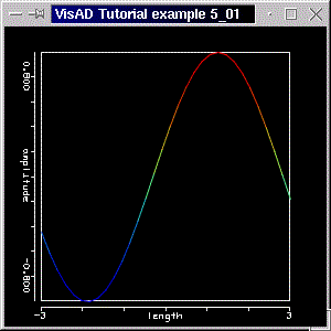
That's exactly what we do in example P5_01.java. We have one array ampVals with the amplitude values and, inside a while-loop, we calculate the values again and reset the samples. To create the animation, we let the user wait a little, by putting the thread to sleep for half second. See how this is done:
// index to count time step
int index=0;
// Loop forever, changing the samples array every time
while(true){
  try{

    // recalculate the values
    for(int i=0;i < nSamples;i++){

      ampVals[0][i] = (float) Math.sin( lenVals[0][i] + (float) index);
    }

    // Update samples
    amp_len_ff.setSamples( ampVals );

    index++;
    Thread.sleep(500);
  }
  catch (InterruptedException ie){
   ie.printStackTrace();
  }

}
As usual, the code for example P5_01 is available here. Run the example with "java tutorial.s5.P5_01". You should get an animated sine wave, of which we made a snapshot like below.

You could try this on the other examples. You could then animate the other lines and points, animate the surfaces and so on.
Yes, but what about the DisplayRealType Animation? What's it good for, if one can animate a display without it? In the next section we turn our attention to "real" animation with VisAD. We extend the MathType of this example, use DisplayRealType Animation and get acquainted with the AnimationControl.
When thinking of animation with VisAD there are two things you should bear in mind. First, whether you can achieve animation by using a loop like in the previous section. This simplifies a lot your application, but, again, it restricts you to "simple" animation, and thus limits your freedom of trying other visualization forms. Secondly, whether your data, that is, your MathType and your domain set will allow it. Regarding this second aspect, your domain set must be 1D, otherwise you cannot map the RealType component of the (non-1D) domain to Animation.
On ther other hand, animation is completely independent of the choice of display. It is as easy (or as difficult, at first) to animate a 3D display, as it is for a 2D display.
Let us consider a MathType like that of the previous section:
Remember, we had there one FlatField, but many sample arrays, which we calculated on-the-fly. Suppose now that we know in advance how those arrays are, that is, we know in advance what values they contain. (Either that, or you let you calculations finish, and then you know how all values are.) Of course we assume that each array has been computed for a given time. In VisAD notation this can be written:( length -> amplitude )
you don't have to call the "time variable" by the name "time". It might just as well be "index", or "year" or "whatever". But "time" seems more appropriate than ever. What we are saying with the VisAD notation should be clear: amplitude is a function of length, but this function is itself a function of time. Please take some time to see how the RealTypes are parenthesized. First the FunctionType ( length -> amplitude ), and then this MathType as a function of time, and all inside parentheses again. That is, two FunctionTypes. Another example would be( time -> ( length -> amplitude ) )
( time -> ( (latitude, longitude) -> ( temperature, pressure, humidity, ... ) ) )
The important thing to realize, is that the time domain must be a 1D-Set. So we start by defining a third RealType, which will be the one for our "time domain". For now we'll call it "minute", and we create it the usual way:
minute = new RealType("minute", SI.second, null);
It's called "minute", it's measured in SI seconds and has "null" default set. We don't want to call "time" for now. We'll do that in the next section. (The point we want to make is that another RealType, other than "Time", can be mapped to the DisplayRealType Animation. VisAD defines some "standard" RealTypes, and Time is one of them.) The next step regards the FunctionTypes. Remember that amplitude is a function of length:
As promised, we make this function a function of minute:func_len_amp = new FunctionType(length,amplitude);
The line above means, that the function func_len_amp is a function of minute. (To make it clear, "range", in the function's name means the range of the current function. Yes, func_len_amp is the range of the function func_t_range, whose domain is minute. We added a "t" to the name of the variable, not to complicate, but only to remind you that there is a "time" somewhere. In the next section minute will be called "time", and then we won't have to change the name.)func_t_range = new FunctionType(minute, func_len_amp );
In all examples you've seen so far in the tutorial, we packed a lot of information inside a FlatField object. Now we're dealing with many such objects. Remember, in the previous section we had one FlatField, but many arrays of samples. Now we have the same data: the same FunctionType (for amplitude and length), the same FlatField and the same arrays of samples. The new thing is that all of those data are a function of another variable, minute. So, how do we pack all this information inside some object? Fortunately FlatField has got a relative, who can handle the situation. We are going to use a FieldImpl (Field Implementation) to hold all the information. FieldImpl is the subclass of Field, it implements the Field interface and extends DataImpl, that is, it's a VisAD Data class. (So far we've only used FlatFields. The main reason for that was the simplicity of the range. FlatField are more efficient than FieldImpls regarding data operation and storage. But because they are specialized, they must impose restrictions on the data type. Their superclass, the FieldImpl, doesn't make such restrictions and is, therefore, capable of more, even though you might pay a price for efficiency. See section 3.9 of the Developers Guide for more details.) Remeber how to create a FlatField?
You needed a FunctionType and a domain Set. For a FieldImpl it's not different:amp_len_ff = new FlatField( func_len_amp, lengthSet);
where timeSet is the domain set and had previously been created withtimeField = new FieldImpl( func_t_range, timeSet);
Note that the domain is 1D!int tSamples = 12; timeSet = new Integer1DSet(minute, tSamples);
So our time domain is called minute, and we wish to map it to Animation. We assume we have 12 arrays of samples, thus the length of the time set. We created a FieldImpl to acomodate all those data. Now we only have to put the individual arrays of samples in the FlatFields and put those FlatFields in the FieldImpl. This is done with a for-loop, for example:
// loop once for all time steps
for(int t=0;t < tSamples;t++){

  // and twice to create some "amplitude" values
  for(int i=0;i < nSamples;i++){

    ampVals[0][i] = (float) Math.sin( (float) lenVals[0][i] + t);
  }

   // and initialize the FlatField with the samples array
  amp_len_ff.setSamples( ampVals );

  // set amp_len_ff as the t-th component of the Field
  timeField.setSample( t, amp_len_ff  );

}
The rest of the application follows the usual pattern. We create some maps, of which only one is worth mentioning:
timeAnimMap = new ScalarMap( minute, Display.Animation );
After adding the maps to the display, we create a data reference:
data_ref = new DataReferenceImpl("amp_len_ref");
(up to now, all data was in a single FlatField. Now we have all data inside a FieldImpl.)data_ref.setData( timeField );
This data reference is added to the display, as usual. Then we must get the AnimationControl from the Animation map, otherwise there will be no animation (the default value for animation is "off"):
That is, get the AnimationControl, and turn animation on.AnimationControl ac = (AnimationControl) timeAnimMap.getControl(); ac.setOn( true );
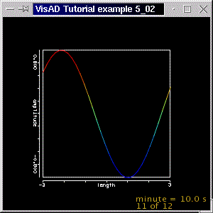
Ready! By running example P5_02 you should get an animation, which resembles the previous example. One difference can be seen in the display: the value of RealType which is mapped to Animation is drawn. That is, the value of minute is shown with corresponding units.
As usual, the code for example P5_02 is available here. Run the example with "java tutorial.s5.P5_02". You should get an animated sine wave, like that of the previous example, which is no wonder, since they have the same values. The "only" difference lies in the MathTypeand in the use of Animation. Below is a screenshot of the current example.
VisAD also provides an AnimationWidget to go together with the AnimationControl. We will soon introduce it. Also note that, although you need a 1D set for the animation domain, the set must not necessarily be an Integer1DSet. We will soon use another 1D set for the time domain.
Now that you've seen what type of data is needed for "real" animation in VisAD, we shall change example 5_02 a little to offer some variations on data depiction.
In the previous section we called "minute" the variable we mapped to Animation. We said, though, that VisAD already defines "Time". So we take the opportunity to use it and to introduce a novel way of creating a RealType.
VisAD keeps a list of all RealTypes within the same Java Virtual Machine, so whenever you create a new RealType, VisAD looks up for already existing RealTypes with the given name. If the name has already been used, and you are trying to create a new RealType with that existing name, than you get a VisADException. We know, that there is such a RealType called "Time", and that's the one we want to use. (Of course, you are free to call it "year", "era", "temp", "tiempo", "Zeit", or whatever you judge best, but "Time", "as such" has already been defined.) So instead of creating it again, we use the static method of RealType class:
time = RealType.getRealTypeByName("Time");
Anyway, in this example we open up another dimension and use a 3D display, rather than a 2D display like in the previous example. As promised in the section title, we map Time ZAxis, just to see something different. Note that we do not add the Animation map to the display, and also have commented out the lines in which the AnimationControl is created (otherwise we'd get a NullPointerException when trying to create an AnimationControl out of a map which is not added to a display).
That is, rather than animating the display, we'll be getting the sine curves stacked up in the z-axistimeZMap = new ScalarMap( time, Display.ZAxis );
Please run the example with "java tutorial.s5.P5_03". The code is available here. You should get a display like the screenshot below.
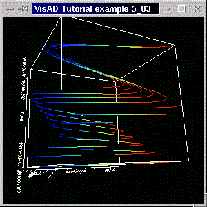
You're seeing the display cube almost from the x-axis. The z-axis, Time, is on the left. You should also try adding to the display the Time to Animation map (and don't forget to uncomment the two lines of code, where the AnimationControl is created and the animation is set on). The lines of code are already in P5_03.java.
Finally note that the ScalarType has an alias(String alias) method. That means you can create a ScalarType like
time = RealType.getRealTypeByName("Time");
You can then refer to the ScalarType Time through its alias Tempus, but the original is still valid.time.alias( "Tempus" ); time.alias( "Khronos" );
In this section we introduce the AnimationWidget. Although you can use AnimationControl to set animation on and off, to set its speed and other parameters, the AnimationWidget provides you with the comforts of a modern UI.
But before we create the widget, we take the chance to use another set for the time set. In the previous examples we had an Integer1DSet as the time set. Now we use a Linear1DSet. Remeber that in a linear set you define the start and end values, as well as the set's length:
We haven't changed the length. We still have the same number of values arrays, 12 in total. Note that our animation starts at 11 s and ends up 12 seconds later, when Time has the value of 23 s. (The actual animation does not necessarily last 12 seconds. In case you want it to last 12 seconds, than you must set the corresponding number of milliseconds per animation frame. You can use the AnimationWidget for that.)timeSet = new Linear1DSet(time, 11.0,23.0, tSamples);
The creation of an AnimationWidget is absolutely no trouble, especially now that you've met a few of its brothers and sisters.
We create an AnimationWidget with the line
where timeAnimMap is the ScalarMap whose DisplayRealType is Animation. We then add the widget to the frame withanimWid = new AnimationWidget( timeAnimMap );
like you'd do with any ordinary Java Component.jframe.getContentPane().add(animWid);
As usual, the code for this example is available here. Run the example with "java tutorial.s5.P5_04". You should get an animated sine wave, like that of example P5_02. The difference is that Time starts at 11 s. Note that the absolute time starts on the 1st of January, 1970, the start value of a Java Date. Below is a screenshot of the current example.
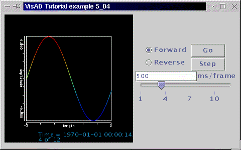
The animation widget has radio buttons for selecting the animation direction and buttons to start, stop or step the animation. A slider shows the current animation step, and you can type in the step interval, in milliseconds.
In the next section we introduce the VisAD DateTime class, which allows you more control over a date format.
In the previous section we used a Linear1DSet to represent the Time values. We said you can use "proper" dates, and we meant that not only you can use a Java Date, but you can also format the way is displayed.
We start off by defining some Java Dates. As you know, the java.util.Date class provides a bunch of deprecated constructors, so we grab a couple of java.util.GregorianCalendars to construct some dates. We do this with
GregorianCalendar startDate = new GregorianCalendar( 1997, Calendar.MAY,  Calendar.DATE);
GregorianCalendar endDate = new GregorianCalendar( 1997, Calendar.MAY, Calendar.DATE + tSamples -1 );
(Please consult the Java Documentation if you are unsure how to create a Date.) We create start and end dates, so that they are in May, in the year 1997, and there are tSamples days between them. This is all arbitrary. You could create two dates separated by tSamples seconds or whatever you need.
The nice thing about java.util.Calendars is that you can set the date format as you please. Please refer to the Java Documentation on how to set your own java.text.SimpleDateFormat. Although this is an optional step, it's most likely that you will want to define your own pattern. In example P5_05 we set a date format with the string:
String myDateFormat = "yyyy/MMMM/dd ";
Remember, we want to input this information into a VisAD data object. The object we have in mind, is, of course, our Linear1DSet. We had start and end values in the constructor of the Linear1DSet, and thus we want to transform those dates above into doubles. For that VisAD provides the DateTime class. You create a DateTime object with a java.util.Date object. You can then format it with your own format pattern, and you can get the double value from it and initialize your Linear1DSet with this value. This is how to do it:
Note that the method GregorianCalendar.getTime() returns an instance of the java.util.Date class. The Linear1DSet is created as usual:// Create a DateTime object and set its date format DateTime dt = new DateTime(); dt.setFormatPattern( myDateFormat ); // initialize the DateTime object with the start/end dates // ...and get the double values from it dt = new DateTime( startDate.getTime() ); double startValue = dt.getValue(); dt = new DateTime( endDate.getTime() ); double endValue = dt.getValue();
There are no tricks in the code. We do everything as usual. The only point to make, is that the Linear1DSet has VisAD's Time as its domain.timeSet = new Linear1DSet(time, startValue, endValue, tSamples);
You can have a look at the code here. Run the example with "java tutorial.s5.P5_05". You should get an animated sine wave, like that of previous examples. Note that the formatted date is shown on the display, as you can see in the following screen shot.
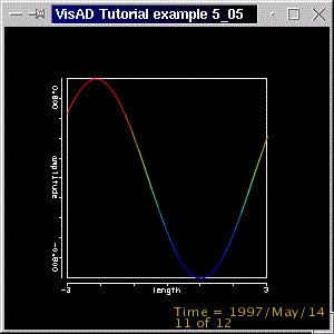
One important thing to realize, is that you can use VisAD's Time without animation. This can be useful when plotting some quantity against time. For example, you could have distance plotted against Time on a 2D display (say, distance on the y-axis and Time on the x-axis). You can actually see in P5_03, that the z-axis is labelled with dates. The Time axis can be labelled with the date format pattern you provide.
In this section we extend the MathType so create an animated surface. We should perhaps define what we mean by "an animated surface". One could think of a surface, whose form changes with the time, but others might only be interested in seeing how some attribute of a surface, say, temperature of the Earth surface, changes over time. For example, think of a surface like a carpet. You could shake it and/or change its pattern according to time. (Very much like as if it gets rugged and fadded with time.) We shall create a MathType which will allow for both. You know you could change the way you visualize your data by changing the ScalarMaps. So we shall provide the basics, and then will leave up to you to decide what's best for yourself.
We simply follow the pattern described in section 5_02, but we assume a more complex MathType, for example, like that of section 4_01. We start with a MathType like
where latlon and altitemp are the domain's and range's RealTupleTypes, respectively. They are related by the FunctionType( ( longitude, latitude ) -> ( altitude, temperature ) )
func_latlon_at = new FunctionType(latlon, altitemp);
This is nothing new. Also remember that the domain set is now 2-dimensional:
latlonSet = new Linear2DSet(latlon, -Math.PI, Math.PI, NROWS,
    					                      -Math.PI, Math.PI, NCOLS);
As usual, we create a FlatField with the FunctionType and the 2D domain set:
latlon_at_ff = new FlatField( func_latlon_at, latlonSet);
The altitude and temperature values must fit inside an array like
Remember that, the "2" as the first array dimension has to do with the fact that the range is 2D, whereas the fact that the domain is 2D is indicated by second dimension of the array, which is given by two values: NCOLS and NROWS. If the range were temperature, only, than we would have an array like double[1][NCOLS * NROWS]. (Of course, you can use float values, too.)double[][] flat_samples = new double[2][NCOLS * NROWS];
The FunctionType func_latlon_at is the range of other FunctionType:
where time is our well known RealType Time, and also the domain of this function.func_t_latlon = new FunctionType(time, func_latlon_at );
The time set is one-dimensional. The Field object is created with the FunctionType func_t_latlon and with the time set:
We loop over the length of the time set, generate altitude and temperature values, set the FlatField with those values, and set the n-th value of the Field with the current FlatField. This is almost exactly what we did in section 2_01 The only difference is an extra for-loop to account for the extra domain dimension:timeSet = new Linear1DSet(time, startValue, startValue + tSamples, tSamples); timeField = new FieldImpl( func_t_latlon, timeSet);
// loop for time steps
for(int t=0;t < tSamples;t++){


// ...and then loop over columns and rows to calculate individual...

  for(int c = 0; c < NCOLS; c++)

    for(int r = 0; r < NROWS; r++){

      // ...altitude
      flat_samples[0][ c * NROWS + r ] = (float)( (Math.cos( t +
                  0.50*(double) set_samples[0][ c * NROWS + r ])  )  ) ;


      // ...temperature	values
      flat_samples[1][ c * NROWS + r ] = (float)( (Math.sin( t +
                   0.50*(double) set_samples[0][ c * NROWS + r ])  ) *
                   Math.cos( (double) set_samples[1][ c * NROWS + r ] ) ) ;


  }

  // set those values in the FlatField
  latlon_at_ff.setSamples(flat_samples);

  // and the FlatField as the t-th Field value
  timeField.setSample( t, latlon_at_ff  );


}
Forget about the individual altitude and temperature values. They vary according to some complicated sine and cosine function, and they where chosen only because they bring some life and color to the surface. You are supposed to provide you our values, anyway.
As usual, the code for example P5_06 is available here. You should get an animated cosine wave, which look likes as if it were flying off in the positive longitude direction. The temperature values also vary with time. Unfortunately we could only make a snapshot of it, so we urge you to run the example with "java tutorial.s5.P5_06".
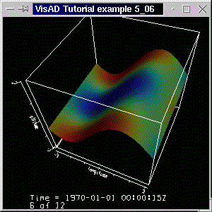
Now that you've seen that an animated 2D cosine wave surface, with a cos(x) times sin(y) as the coloring attribute looks impressively like a flying magic carpet, of which dust is being shaken off, we may move on. Note, however, that you can create a third type of animated surface by rotating the display in steps. (Hint: the method DisplayImpl.make_matrix(), the Projectioncontrol and/or VisAD examples 57 and 58.) In the next section we shall introduce another widget, the VisADSlider, and shall use a SelectValue map.
The VisADSlider is like a specialization of a Java Slider for use in VisAD. The VisADSlider can be linked to a Real through a DataReference, so that the value of the Real changes according to changes in the VisADSlider. Alternatively, the VisADSlider can be initialized with a SelectValue map, so that the value of the RealType of the ScalarMap can be set with the slider. But what's a SelectValue map? Remember when we used the AnimationWidget in section 5_04? It too had a slider, and each time this slider moved, the value of the Time changed. This is almost the same as saying that we had a ScalarMap whose RealType was Time and whose DisplayRealType was SelectValue. Whenever we had a time step, the value of time was "selected" again. SelectValue only applies to 1D domains, like it is the case of Animation.
Our starting point is the previous example. We declare another ScalarMap, and create it with
Here we finally meet the DisplayRealType SelectValue. Note that the ScalarType associated with this map is Time, which is the domain of the 1D set. We add this map to the display, as usual. Next we create the VisADSlider with the above map:selValMap = new ScalarMap( time, Display.SelectValue );
vSlider = new VisADSlider(selValMap);
We then add this slider to the window where we had put the display. The result can be seen in the screen shot below.
As usual, the code is available here.
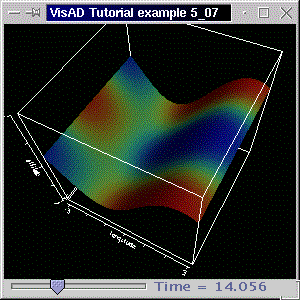
By moving the slider knob you set the value of Time. The display is then automatically updated. Note on difference to the slider of the AnimationWidget: while that set the animation step, the VisADSlider sets the value of a Real. You can see this value indicated by the slider label.
But the VisADSlider is not really an alternative widget to the AnimationWidget. You can also use the VisADSlider as an input widget. There are also other constructors for the slider, and in the next section we shall meet another one of them.
In this section we introduce three things: the ValueControl, another constructor for the VisADSlider and a Cell, or, more precisely, a CellImpl.The first two of them shouldn't cause any strong feelings amongst the readers. Although up to now we've only mentioned Cells in section 1.1, it is very important class. A Cell is very much like a spreadsheet cell. A Cell is an interface that extends Action. It can be linked to data through a DataReference, so that it performs some action whenever any of its linked data object changes. In practice, you create an instance of CellImpl and override the method doAction().
This example is a little variation on the previous. We still have the SelectValue map and get its ValueControl with
We've had to declare it "final", beacuse we are going to use it inside an inner class, the CellImpl. (Note that when you want to change the selected value, you call ValueControl.setValue( double value ).final ValueControl valControl = (ValueControl) selValMap.getControl();
Next thing we do is to create a DataReference to link the VisADSlider to the Cell.
final DataReference value_ref = new DataReferenceImpl("value");
This constructor takes the newly created data reference as an argument, as well as minimium, maximum and start values, the RealType and a string to be displayed on the slider.vSlider = new VisADSlider(value_ref, 10, 22, 12, time, "Time (s)");
As said, we use a CellImpl to perform an action whenever the data object it's linked to changes its value. In our case, this is the value of Time. The new value of Time will be given by the current value of the slider. Whenever you move the slider, the cell listens and takes some action. Inside the doAction() method, we get the value of the data reference (remember, this reference has been used in when constructing the slider), and set the Time value to be the value we got from the slider. See how this is done:
CellImpl cell = new CellImpl() {
  public void doAction() throws RemoteException, VisADException {

    valControl.setValue(((Real) value_ref.getData()).getValue());
  }
};
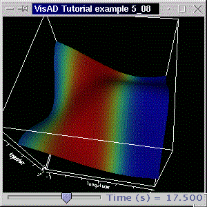
What we've done in this example is similar to what we did in the previous. Whereas you'd rather implement things like done in that example, we wanted to show an alternative method. We have also introduced the ValueControl, we've shown how to use the VisADSlider in a different manner, and we've also introduced a Cell. In the next chapter we will come across Cells more often. For now you can run the example with "java tutorial.s5.P5_08". The code is available here. You should get a display with a surface. The surface data is exactly the same as that of the previous example, we've only swapped the ZAxis and the RGB maps, to get a different image. See the screen shot below. Of course you could try with other maps, too. For example, try to mapping Time to the z-axis and/or to RGB.cell.addReference(value_ref);
In the next section we change the subject a little. We shal talk more about MathType structure and shall use a VisAD Data Form as an example.
Until now we've built MathTypes according to our needs. We've defined RealTypes, related them with FunctionTypes, created data Sets and Fields. But what if we are given a pre-defined MathType? Or more precisely, is it possible to analyze a MathType in some (recursive) way in order to extract its components?
You might have read or heard that VisAD provides various data adapters. (You should have a look in package visad.data and in its subdirectories. Section 7 of the VisAD Java Component Library Developers Guide describes some data adapters and other aspects of them.) In this section we analyze the data provided by one such adapter, the GIF/JPEG Adapter.
The starting point for our example is to consider how a GIF/JPEG image is described in VisAD. Although the following structure is not the only one possible structure for such an image, it corresponds to the way most people would imagine it:
That is, the domain of a color image is 2D, and its range is 3D. As said, this is not the only possible representation; it is, nevertheless, a intuitive one. Note that the above representation implies an Integer2DSet as the domain set, because rows and columns are always integer. But what would that be in case, say, of a satellite image? Each image pixel would represent a "point" (or a little area, to be more precise), and thus be given by coordinates. In this case, it'd be prefereable to have a Linear2DSet. The number of rows and columns of the above set would still be given by the lengths of the set (one for each domain dimension).( (Column, Row) -> (Red, Green, Blue) )
To turn back to the problem, let us consider we're opening some data with a VisAD adapter. As said, we use a GIFForm:
(The GIFForm actually uses a GIFAdapter. The VisAD Form class is the superclass of all VisAD data adapters. Please refer to the Developers Guide for more information.)GIFForm image = new GIFForm();
To get the actual data from the image, we do:
The Form.open( String filename ) method returns a VisAD Data object. We are assuming that the string args[0] is the name of some image. Well, suppose you don't have a clue what the MathType of your Data really looks like, you could get a hint withDataImpl imageData = image.open(args[0]);
which will output the MathType in the usual VisAD notation. The above will produceSystem.out.println(imageData.getType().prettyString());
So you see that the MathType of the image is a FunctionType. To get the FunctionType we then do:( (ImageElement, ImageLine) -> (Red, Green, Blue) )
See how we cast a type on the image type. (The method returns a MathType. So we cast the MathType into a FunctionType.) So we know how the GIFAdapter represents the image. Now that we have the whole MathType, we can start constructing other MathTypes to mirror the image structure. We are going to get the domain and the range of the FunctionType above. Then we'll get the individual components of those RealTupleTypes, and finally we are going to use them to construct some ScalarMaps. This is all very simple. Starting with the FunctionType, get the domain and the range:FunctionType functionType = (FunctionType) imageData.getType();
Both of them are RealTupleTypes. To get the individual components, that is, the RealTypes, we do:RealTupleType domain = (RealTupleType) functionType.getDomain(); RealTupleType range = (RealTupleType)functionType.getRange();
in our application, longitude and latitude are RealTypes which correspond to ImageElement and ImageLine, respectively. We create from Red, Green and Blue the following types:longitude = (RealType) domain.getComponent(0); latitude = (RealType) domain.getComponent(1);
Note that you can get the dimension of a RealTupleType withredType = (RealType) range.getComponent(0); greenType = (RealType) range.getComponent(1); blueType = (RealType) range.getComponent(2);
In this case, domDim is the domain dimension. This method is useful when you don't know the size of the domain and/or range.int domDim = domain.getDimension();
We then create some ScalarMaps with the RealTypes we got above. For example,
We need a display, and we add the necessary maps to it. We also create a data reference, and set its data with the image data:greenMap = new ScalarMap( greenType, Display.Green );
Remember, we got imageData when opening the file with the GIFForm.data_ref.setData( imageData );
Running the example with "java tutorial.s5.P5_09 image_name" will load the GIF or JPEG image and display it on a 2D display. The code is available here. Below is a screen shot of the example.
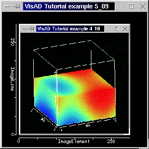
In this example we got data from a VisAD Form, "reconstructed" it and then we displayed it. Surely we got some help with the MathType.prettyString() method. That wasn't very elegant, though helpful. Section 7.1 of the Developers Guide describes a way to recursively analyze a MathType structure. In section 3.1.15 you'll find another example of a MathType analysis. You might also be interested to know about the following MathType method.
This method creates a MathType from a string (in VisAD notation).myMathType.stringToType( String s );
Before we move on, we'd like to mention another way to get information about VisAD Data. The visad.jmet.DumpType class has two static methods for displaying information about VisAD Data or a MathType. In the next section we will use one of them and we'll also return to animations.
In this section we use the previous example to load and animate a series of images. This example is introducing nothing new. It combines the previous exammple with the others in this chapter, especially example 5_06.
Example 5_06 is our starting point. We load an image, extract its MathType, create ScalarMaps, etc. To animate the series of images, we create a RealType and a domain set:
time = RealType.getRealTypeByName("Time");
Again, no surprises here. The domain set is timeSet, and it'll hold a number nImages of images (this value will be determined by the number images given in the command line). The domain set is 1D, as usual, an it's an Integer1DSet for no special reason. You can use other 1D sets, like we did in other examples in this section.timeSet = new Integer1DSet(time, nImages);
We need to the image's MathType, which we had called functionType, as a function of Time:
The Field is constructed with this FunctionType and with the domain set.func_t_latlon = new FunctionType(time, functionType);
Now that we have the Field, we can start setting its data. We'll do it for every image, of course. As we've already got the data from the first image, which we had opened to analyze the MathType, we put it into the Field:timeField = new FieldImpl( func_t_latlon, timeSet);
The other images will be opened and put into the Field with a for-loop. Now that we have data in a complex MathType, we can call the following static method of visad.jmet.DumpType, which will recurse through the MathType and display information about it.timeField.setSample(0, imageData);
Watch out for the displayed information. (You can redirect this information to some other OutputStream.) The methodDumpType.dumpMathType( func_t_latlon, System.out);
will display list out information about a VisAD Data object. (Note that visad.jmet.DumpType also has a main method, which can be used to check data VisAD knows how to read, that is, data for which an adapter exists.)DumpType.dumpMathType( Data d, java.io.OutputStream os);
We then set and add the data, that is, the Field, to the display:
data_ref = new DataReferenceImpl("image_ref");

data_ref.setData( timeField );

display.addReference( data_ref );
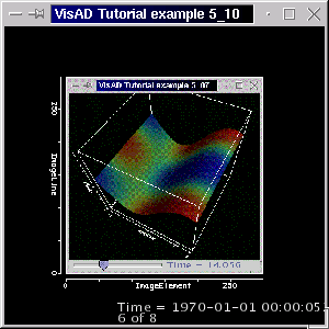
Note that when loading a large number of images and/or loading large images, with should add the "-mxMMMm", where "MMM" is the memory size in MB, option to the command line, otherwise you may run out of memory.
As warned, this example brought nothing new. You might wonder, though, what kind of data object an image represents. We know from analyzing its MathType what structure it has. But we haven't mentioned what sort of data object is behind it. Well, hopefully you won't be surprised to know it's a FlatField. As said, there's nothing new in this example. In a sense, it's a variation of example 5_06, where we had the animated surface. One little difference, though, is that whereas in section 5_06 we had one FlatField object and many different values arrays, here we get a different FlatField each time we open an image. That is, the MathType is always the same, but the FlatField isn't. That means you can load images of different sizes, and set them as the i-th Field value.
Because an image is a FlatField (and also a Field; remember, FlatField extends Field), you can call its Field methods. In particular we want to mention
which will return a Linear2DSet, andFlatField.getDomainSet();
which will return the samples values. In the case of a GIF/JPEG image, it'll return an array double[ 3 ][ NROWS * NCOLS ], with the pixel values. Of course, the "3" means that we have three range components: red, green and blue.FlatField.getSamples();
Now that you can animate you progress through the tutorial, by calling P5_10 with the screenshots as parameters, it's time to move on and get to know another widget.
In this section we introduce another widget, the MappingDialog. The MappingDialog is not in the package java.util like most of the other widgets. It actually belongs to the VisAD SpreadSheet, so it resides in the java.ss package, like other VisAD SpreadSheet components. The MappingDialog allows you to select how each ScalarType of a given MathType will be mapped. After you've selected how you want your mappings, the MappingDialog creates the ScalarMaps for you. Then you only have to add those to your display. To show how to do it, we start off with the previous example. We'll need a Java Button to call the MappingDialog.
Remember from the previous section, that we opened a number of images, got all the data, that is, a number of FlatFields, and packed all this data inside a Field object. The domain of this Field was Time, and the domain set was a 1D set, with length equal to the number of images. The MathType was like the following:
Recall that we created a ScalarType for each of the RealTypes above. It was simple, but a quite cumbersome. We mentioned a recursive way to parse the MathType tree and analyze it. However, if you want to parse the MathType structure to create ScalarMaps only, then you don't have to bother about analyzing MathTypes. You might be happy to know that the MathType class has a method MathType.guessMaps( boolean threeD ). And you might have guessed it right: the method guesses at a set of "default" mappings for a given MathType. In the current example we use it:( Time -> ( (ImageElement, ImageLine) -> (Red, Green, Blue) ) )
That is, on the right we get the MathType of the data (remember, all data is a Field of images, which we called timeField), and then we call the method guessMaps( true ) (we are assuming 3D data, so the argument "true"). The method returns an array of ScalarMaps, so we have defined such an array: sMaps. Well, we have data, and we have ScalarMaps, what else do we need to visualize it? We need a DataReference and a display. And that's about it.sMaps = timeField.getType().guessMaps( true );
In this example we create a convenience method to add an array of ScalarMaps to a display, because we are going to do this often. We also get an array of ScalarMaps from the MappingDialog. The method does another important thing: it checks whether any of the ScalarMaps in the array is an Animation map. If so, then it creates an AnimationControl from it, and starts the animation. (Remember from section 5_02, that animation is turned off by default.) The method is as follows:
  private void addAllMaps( DisplayImpl d, ScalarMap[] sm){

    for(int i=0;i < sm.length;i++){

      try{

        d.addMap( sm[i] );

        if( sm[i].getDisplayScalar().equals(Display.Animation)){

          ac =(AnimationControl) sm[i].getControl();
          ac.setOn(true);
          ac.setStep(1000);
        }

      }
      catch(VisADException ve){
        // do something...
      }
      catch(RemoteException re){
        // do something...
      }
     }
  }
To create a MappingDialog we use the constructor:
The arguments are the parent frame, the data object, the initial ScalarMaps, and whether it allows alpha and 3D mapping, respectively. You may also initialize the MappingDialog with an array of data objects. Please refer to the documentation. But in this example we only dealing with one (big) data object, the timeField.md = new MappingDialog(jframe, timeField, sMaps, true, true);
As said, we use a JButton to make the MappingDialog visible. The JButton performs the following action when clicked:
      public void actionPerformed(ActionEvent E){
        try{

          // Call the mapping dialog and get the chosen maps from it
          md.display();

          sMaps = md.getMaps();

          // Clear display
          display.removeAllReferences();
          display.clearMaps();

          // Add chosen maps
          addAllMaps( display, sMaps);

          // Add the data reference again
          display.addReference( data_ref );

        }
        catch(VisADException ve){ ve.printStackTrace();
        }
        catch(RemoteException re){ re.printStackTrace();
        }

      }
    });
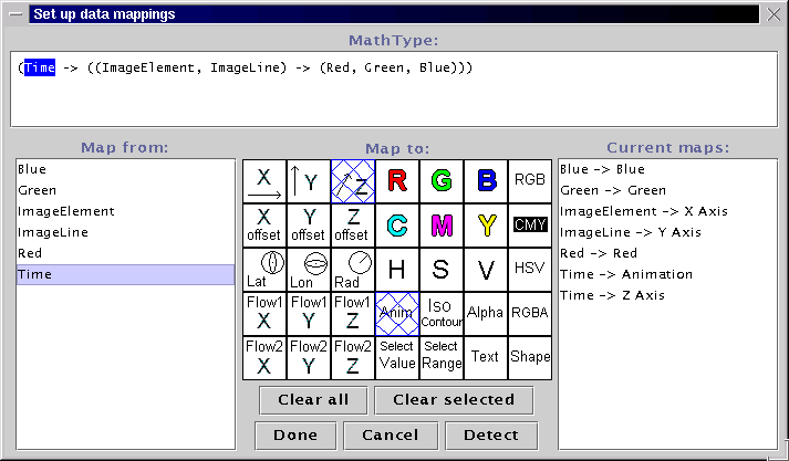
The MappingDialog interface is divided into five areas. On the top you can see the MathType of your data, in VisAD notation. On the left, you have a list of ScalarTypes. In the middle you see a number of icons, which represent the DisplayRealTypes. Below them there are buttons for clearing up the selection, for detecting maps, for cancelling and for closing the dialog. The last will create an array of ScalarMaps. Finally, on the right you see the current selections. See for example, that we have selected the RealType Time (either by clicking on "Time" at the top area or at the left area). You can see how Time will be mapped by either checking the hachured icons or by reading the current maps on the right area.
After clicking on the "Done" button, you can get the chosen maps with
Now we have the new maps in our ScalarMap array. We must clear the display, before we add the new maps. First we remove the single data referencesMaps = md.getMaps();
Then we clear the maps:display.removeReference( data_ref );
We are then ready to reconstruct the display. We add all maps with our convenience method and then we add the data reference:display.clearMaps();
You can have a look at the whole code here. Run the example with "java tutorial.s5.P5_11 image_1.gif image_2.gif ...". You can also run it with JPG images. Below is a screenshot of the application.addAllMaps( display, sMaps); display.addReference( data_ref );
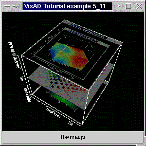
The application starts with a set of "guessed" maps. They are
but the screenshot shows the mapping:Blue -> Blue Green -> Green ImageElement -> XAxis ImageLine -> YAxis Red -> Red Time -> Animation
Note that not all mappings are valid. Please refer to the Appendix A and to section 4.1 of the Developers Guide for more information. Also, when adding maps to a display, you might want to check for other ScalarMaps in order to construct some special widget. For example, you might want to check for a SelectValue map to add a VisADslider, check for a SelectRange and add a SelectRangeWidget and/or add some RangeWidgets.Blue -> Blue Green -> Green ImageElement -> XAxis ImageLine -> YAxis Red -> Red Time -> ZAxis
Also note that, when using a VisAD adapter, you only need to get the data, get its the MathType, let your application guess the maps for the MathType, add those maps and by using a data reference, you can construct a display with very few lines of code.
When clearing a display you can remove all data references at once with
Also note that, if you want to turn some data on or off, you might do it without clearing the display. Just dodisplay.removeAllReferences();
DataReference data_ref = new DataReferenceImpl("ref");
data_ref.setData(data);
DataRenderer renderer = new DefaultRendererJ3D();
display.addReferences(renderer, data_ref);
. . .
renderer.toggle(false); // turn off depiction of 'data'
. . .
renderer.toggle(true); // turn depiction of 'data' back on
We come to the end of this chapter. By now you should be able to contruct some complex MathTypes, to create quite a few different displays and to use a number of widgets to interact with your display and with your data. Of course, there's more to come. Especially on the subject of interaction. So, let us move on to the next chapter, where we consider interaction in more detail.