 |
Other sites |
Microphysical Data
The bulk of our data are derived from aircraft measurements obtained in field campaigns over the past several decades. These data are analyzed and provided by Dr. Andrew Heymsfield and his colleagues, Dr. Carl Schmitt and Aaron Bansemer, all at the National Center for Atmospheric Research.
For our use in developing ice cloud single-scattering property models, we filtered each data set so that the cloud temperature T ≤ -40˚C. We did this to ensure that we were working with ice cloud data. Each individual measurement is derived from 5 seconds of probe data and includes the gamma distribution coefficients (slope, intercept, dispersion) necessary for calculating the particle size distribution (PSD), the temperature at which the measurement was made, the ice water content (IWC), the median mass diameter, and the maximum diameter that should be permitted in the PSD.
If there is interest in working with a more complete, unfiltered data set for any or all of these campaigns, send a request by email to the NCAR scientists listed above.
Field Campaigns and Access to Microphysical Data
The data for the SCOUT, CRYSTAL-FACE, and Pre-AVE campaigns were revised (August, 2011) to reflect better consistency between probes and to account for refinement of processing procedures. New data are now available from the TC-4 and MPACE campaigns. The data from these campaigns provide the best data for ice clouds having very low IWC values, and have the smallest effective diameters. The number of PSDs has increased for each of these campaigns over what we reported previously, and the quality of the data are much improved.
Access to each of the individual sets of microphysical data are provided by the "Download Data" button at the top of the page. Note that there is a new system in place at SSEC and we now ask that you register before downloading data - all we ask for is your name and email address. Since there will be updates in the future, we hope that you will permit us to include you on an email list so that we can send a brief note with what has changed in each subsequent version. So when you register, there will be a box that asks you whether you want to be on an email list - it is voluntary on your part.
These microphysical data files are not currently in a format that supports metadata like netCDF, but are simply text files. Each line of data contains the following information in order: cloud temperature (˚C), slope, intercept, dispersion, ice water content (g m-3), median mass diameter (cm), and the maximum diameter (cm) that should be used in building the size distribution. The particle density calculated in each size bin by the modified gamma distribution equation on this page has units of #particles per cm3 per cm.
Field Campaign |
Year |
Location |
# of 5-sec PSDs |
Probes |
| ARM-IOP | 2000 |
Oklahoma, USA | 1420 |
2D-C, 2D-P |
| TRMM KWAJEX | 1999 |
Kwajelein, Marshall Islands | 201 |
2D-C, HVPS |
| CRYSTAL-FACE
--WB57 |
2004 |
Florida area, over ocean | 221 |
CAPS, VIPS |
| SCOUT | 2005 |
Darwin, Australia | 358 |
FSSP, CIP |
| ACTIVE-Monsoons | 2005 |
Darwin | 4268 |
CAPS |
| ACTIVE-Squall Lines | 2005 |
Darwin | 740 |
CAPS |
| ACTIVE-Hector | 2005 |
Darwin | 2583 |
CAPS |
| MidCiX | 2004 |
Oklahoma | 2968 |
CAPS, VIPS |
| Pre-AVE | 2004 |
Houston, Texas | 99 |
VIPS |
| MPACE | 2004 |
Alaska | 671 |
2D-C |
| TC-4 | 2006 |
Costa Rica | 877 |
CAPS, PIP |
To Build a Particle Size Distribution from the Data...
To build a particle size distribution given the slope, intercept, and dispersion, here's a snippet of fortran code to build a single size distribution (assuming that you have set up a variable that contains the desired size bins, each with a representative diameter):
open(10,file='TC4_microphysics.dat',status='unknown')
read(10,140) temp,slope,intercept,dispersion,icewatercontent,Dmedianmass,Dmax
do bin=1,maxsizebins
maxdim = maxdimension(bin)
if (maxdim .le. Dmax) then
binweight(bin) = intercept*exp(-maxdim*slope)*maxdim**dispersion
! binweight provides the particle density in units of number of particles per cm^3 per cm
else
binweight(bin) = 0.
endif
enddo ! end loop in bins (size distribution)
close(10)
Documentation of the Microphysical Data
Details of the measurements and data reduction are provided in a publication currently under review in the Journal of Atmospheric Sciences. Please contact Andy Heymsfield, Carl Schmitt, or Aaron Bansemer at NCAR for the latest version of this paper as it wends its way through the review process.
Heymsfield, A. J., C. Schmitt, and A. Bansemer, 2013: Ice cloud particle size distributions and pressure dependent terminal velocities from in situ observations at temperatures from 0˚ to -86˚C. J. Atmos. Sci., 70, 4123-4154.
Microphysical Probes
The table below lists the usable size ranges for the 2D-type probes. The PIP's nominal size range (width of array) is 100-6400 microns, but the 'usable' size range is more like 1000-10000 microns. The small end (<1000um) is better covered by the CIP or 2DC, and the large end is bigger since we allow partially imaged particles. The CPI data are not used to create any of the PSDs but images from the CPI are available.
Acronym |
Full Probe Name |
Usable Particle Size Range |
| CPI | Cloud Particle Imager | 20-2000 μm |
| CAS | Cloud, Aerosol, and Precipitation Spectrometer | 2-50 μm |
| CIP | Cloud Imaging Probe | ~100-1600 μm |
| PIP | Precipitation Imaging Probe | 1000-10,000 μm |
| FSSP | Forward Scattering Spectrometer Probe | 2-50 μm |
| VIPS | Video Ice Particle Sampler | ~10-350 μm |
| SID | Small Ice Detector | 1-60 μm |
| 2D-C | Two-dimensional Cloud Probe | ~100-1000 μm |
| 2D-P | Two dimensional Precipitation Probe | 1000-10,000 μm |
| HVPS | High volume precipitation sampler | 1000-50000 µm |
Particle Size Distributions
Particle size distributions (PSD) are parameterized in the form of gamma distributions of the form:
![]()
where Dmax is the particle maximum dimension, n(Dmax) is the particle concentration per unit volume, N0 is the intercept, λ is the slope, and µ is the dispersion. This relationship reduces to an exponential distribution when µ = 0. The values for the intercept, slope, and dispersion were derived for each PSD by matching three moments; in this case, the first, second, and sixth moments were chosen as this set provided the best fit over the measured particle size range. The data are filtered by cloud temperature (T≤-40˚C) to ensure that the particle phase is unambiguously ice. After filtering, more than 14,000 PSDs are available for study. The data were collected from aircraft cloud probes as listed above. Each PSD from the aircraft observations represents a 5-second average, corresponding to about 700m of aircraft movement.
Habit Distributions
In the Version 1 and Version 2 models, insufficient consideration was given to the prescription of habits as a function of maximum diameter. The habits did not change smoothly with size leading to abrupt changes from one set of habits to another. Such abrupt changes can affect the single-scattering properties in ways one might not expect. The smallest particles were predominantly droxtals, which have very unique scattering properties. It is difficult to know, at this point anyway, how common the droxtal particle is. The CPI does not have the resolution to resolve this issue. Also, the SID-3 provides a scattering pattern but more work needs to be done to relate the scattering pattern to a particular type of habit such as the droxtal. For the moment, we are not relying so much upon the droxtal for the smallest particles in a given size distribution.
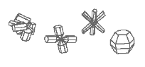
For this new generation of models, a new approach is implemented to assign a more sensible habit mixture as a function of particle maximum diameter. The habits now change smoothly as a function of particle size, and thought has been given in particular to the habit mixture assumed for the smallest and largest particles in a given distribution. For Dmax ≤ 10 µm, the particles are assumed to be droxtals and solid columns. For 10 µm < Dmax ≤ 50 µm, the fraction of droxtals tapers off quickly with particle size, with increasing fractions of solid columns, hollow columns and plates. Mid-sized particles include hollow and solid columns, hollow and solid bullet rosettes, small/large aggregates of plates, and a very small fraction of aggregates of columns. Columnar particles and plates are phased out by the time the maximum diameter reaches 500 µm. The largest particles are composed of hollow and solid bullet rosettes, aggregates of columns (only a very small fraction) and aggregates of plates.
Note: if you have questions or find problems, please let me know (send note to Bryan Baum) so I can look into the issue. If there is a problem, I want to get it fixed.