
Data Fusion: Imager and Sounder
Potential sensor combinations: VIIRS and CrIS; MODIS and AIRS; AVHRR and IASI; AVHRR and HIRS
What do we mean by data fusion? Construction of high spatial resolution IR band radiances (see Weisz et al. 2017 for more details) consists of two steps: (1) performing a search for N sounder FOVs (here N = 5) for each imager pixel using a k-d tree search algorithm on both high spatial resolution and low spatial resolution split-window imager radiances, and (2) calculating the convolved sounder radiances for each of the 5 sounder FOVs selected for each imager pixel. To reduce confusion between the imager and sounder spatial resolution, we use “pixel” for the imager and field of view (FOV) for the sounder.
For a bit more detail regarding step 1: high spatial resolution VIIRS IR window band radiances are spatially downgraded to match the lower spatial resolution of CrIS using geographic colocation information from both instruments. What we mean specifically is that with our geolocation routine, each CrIS field of view (FOV) has a set of VIIRS pixels collocated with it, and the VIIRS 11- and 12-µm radiances are averaged to provide a mean value for the CrIS FOV. Only VIIRS data and VIIRS-CrIS geolocations are used for this process. Both the high spatial resolution (VIIRS) 11- and 12-µm radiances and low spatial resolution (also from VIIRS) 11- and 12-µm radiances at the CrIS spatial resolution are then used to build a function that maps each VIIRS pixel to 5 nearby CrIS FOVs that have similar radiances. A k-d tree approach is used (there is a highly optimized version in Matlab and Python) to select the 5 CrIS FOVs for each imager pixel in the VIIRS 6-minute granule. Specification of N is an arbitrary number that can be changed as desired; to date 5 CrIS FOVs per VIIRS pixel has proven to be sufficient in our testing and validation work.
In step (2), we construct radiances for the N CrIS FOVs selected for each imager pixel. A set of response functions is applied to the hyperspectral radiances for each of the selected CrIS FOVs. For a given spectral band response function, the CrIS radiances are integrated to provide a spectral band radiance. The 5 values of the spectral band radiances are averaged, with no weighting, and the mean value is reported for that pixel. Any number of response functions may be applied, as long as they are contained within the spectral range measured by the CrIS sensor.
Granule examples:
An example is shown in Figure 1 for the case of a 5-minute granule on April 17, 2015 at 1435 UTC over the eastern Atlantic Ocean. In this scene (Fig. 1a), high clouds are white, low clouds are dark grey, and ocean is dark, i.e., cold targets are white and warm targets are dark. The range of radiances is from 2 to 6 W m-2 str-1 µm-1. The 13.3-µm radiances shown in Fig. 1b are constructed from MODIS and AIRS data (See ATBD or Weisz et al. (2017) for details). Note that the (measured – constructed) radiance differences in Fig. 1c are generally less than ±0.05 W m-2 str-1 µm-1 within the AIRS swath. Outside of the AIRS swath (denoted by the red lines in Fig. 4d), there tends to be a negative bias except when there is a cloud. The primary reason for the bias when there is no high cloud present is that we are not accounting for limb darkening outside of the AIRS swath, i.e., the absorption is increasing with path length. This could be corrected with use of a radiative transfer model but this has not yet been implemented. Fig. 1d shows the average distance between the 5 AIRS FOVs selected for each MODIS pixel. Within the sounder swath, the distances are generally less than 200km, while higher outside the swath as expected. Further details may be found in our Algorithm Theoretical Basis Document (ATBD).

Figure 1: (a) Measured MODIS Band 33 (13.3-µm) radiances from a 5-minute granule on April 17, 2015 at 1435 UTC over the eastern Atlantic Ocean. High clouds are white, low clouds are dark grey, and ocean is dark. (b) Constructed MODIS 13.3-µm radiances, (c) pixel-level (measured – constructed) 13.3-µm radiance differences, and (d) mean distances between the 5 AIRS FOVs and the MODIS pixels. Note that within the AIRS swath (red lines), the mean distances are generally less than 200 km, while outside the AIRS swath, the distances increase as expected.
The next step in the process is to apply the fusion approach to VIIRS and CrIS. Figure 2a shows the MODIS granule recorded on April 17, 2015 at 1435 UTC and the constructed 13.3-µm image based on VIIRS and CrIS at 1440 UTC is shown in Fig. 2b. The MODIS and VIIRS sensor overpasses are within 5 minutes of each other for this scene. The similarity of the detailed radiances between the two scenes is remarkable. Note that the constructed 13.3-µm channel covers the complete swath of the 750 m VIIRS measurements. Because the CrIS swath is narrower than the VIIRS swath, the constructed radiances are expected to be somewhat unreliable in the part of the VIIRS swath that lies outside the CrIS data. In the comparison with MODIS, there tends to be a warm bias in the constructed radiances for the non-cloudy pixels outside of the AIRS swath, i.e., the constructed MODIS radiances are higher than the measurements. However, there are cloudy pixels where the opposite is true, i.e., the constructed MODIS radiances are lower than those measured.

Figure 2: a. Measured MODIS Band 33 (13.3-µm) radiances from a 5-minute granule on April 17, 2015 at 1435 UTC over the eastern Atlantic Ocean. High clouds are white, low clouds are dark grey, and ocean is dark. (b) A scene constructed from VIIRS+CrIS data from an overpass about 5 minutes later than the Aqua overpass.
Global examples:
We further investigate the cold bias evident in the constructed radiances that are outside of the sounder (AIRS) swath. A full day of MODIS radiances are constructed and the nighttime ‘real-constructed’ radiance differences are shown in Figure 8. While not shown, the daytime results are similar. The imagery based on the measured 13.3-µm radiances is shown in Fig. 3a and the (real-constructed) 13.3-µm radiance differences are shown in Fig. 3b. As with the single granule shown in Fig. 2, there is a negative radiance bias outside of the AIRS swath where the fusion algorithm is basically extrapolating results, and the chosen FOVs for each pixel outside of the imager swath may not be very closely matched in radiances or situated closely to the pixel. If the imager sensor zenith angle is limited to ±57˚ as shown in Fig. 3c, most of the negative bias is removed from the scene. Where AIRS and MODIS overlap, the radiance differences are generally very small, with a slight increase related to cloud structure as shown in Fig. 2. We note in particular that there is no apparent issue in moving from land to ocean regardless of the land type, nor in moving from snow/ice to water at high latitudes. To summarize, the construction of a 13.3-µm channel seems to offer few artifacts, the radiance differences are small regardless of the surface, but increase slightly within a highly variable cloud field.
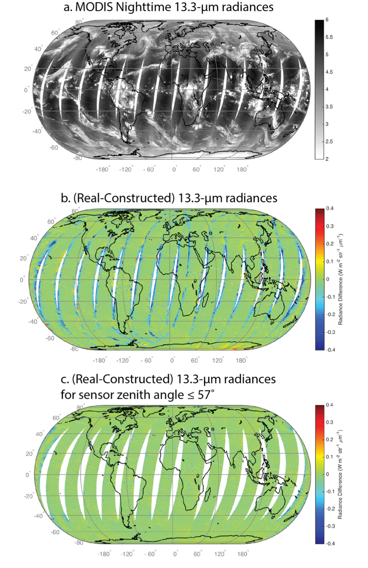
Figure 3: (a) Measured MODIS Band 33 (13.3-µm) radiances for April 17, 2015. High clouds are white, low clouds are dark grey, and ocean is dark. (b) (measured – constructed) 13.3-µm radiance differences for the full MODIS swath. Note that outside the AIRS swath, the constructed radiances tend to become colder leading to a negative radiance difference. (c) (measured – constructed) 13.3-µm radiance differences for the MODIS swath limited to sensor zenith angle ≤ 57˚.
Figure 4 shows daytime results for the MODIS water vapor band 27 (6.72 µm). The grayscale MODIS radiance measurements are shown in Fig. 4a. Figure 4b shows radiance differences (measured-fusion) based on MODIS for a swath limited to 57˚ in sensor zenith angle. The regions with more variability tend to occur over land and are associated with clear-sky conditions, but the differences are still generally low. This variability may be related to surface emissivity differences in the 11- and 12-µm bands, but this is still under investigation. The fusion process is applied to VIIRS+CrIS in Fig. 4c, again with the VIIRS swath limited to the extent of the CrIS swath at a sensor zenith angle of about 60˚. The VIIRS fusion band image shown in Fig. 4c shows remarkable similarity to the measurements in Fig. 4a, at least in the “big picture”. However, there are differences that become more apparent under scrutiny, such as the inability to capture features that have sharp gradients such as dry slots (higher latitudes). The use of sounder data tends to smooth out the sharp features that may be in the higher spatial resolution imager data. Additionally, water vapor can change rapidly with height in the troposphere, and this may also be an aspect that the fusion approach does not capture adequately.

Figure 4: (a) Measured MODIS Band 27 (6.7-µm) daytime radiances for April 17, 2015. (b) MODIS Band 27 (measured – constructed) 6.7-µm radiance differences for the MODIS swath limited to sensor zenith angle ≤ 57˚. (c) Constructed 6.7-µm radiances for VIIRS based on CrIS data, for that portion of the VIIRS swath where there is complete CrIS coverage, i.e., sensor zenith angle ≤ 60˚. From Weisz et al. (2017).
Figure 5 shows daytime results for MODIS carbon dioxide band 35 (13.9 µm). This is one of the key bands used in the MODIS Collection 6 CO2 slicing algorithm to infer cloud top heights. The grayscale MODIS radiance measurements are shown in Fig. 5a. Figure 5b shows radiance differences (measured-fusion) based on MODIS for a swath limited to 57˚ in sensor zenith angle. The regions with more variability tend to occur over land and are associated with clear-sky conditions, but the differences are still generally low. The fusion process is applied to VIIRS+CrIS in Fig. 5c, again with the VIIRS swath limited to the extent of the CrIS swath at a sensor zenith angle of about 60˚. The VIIRS fusion band image shown in Fig. 5c shows remarkable similarity to the MODIS measurements in Fig. 5a.
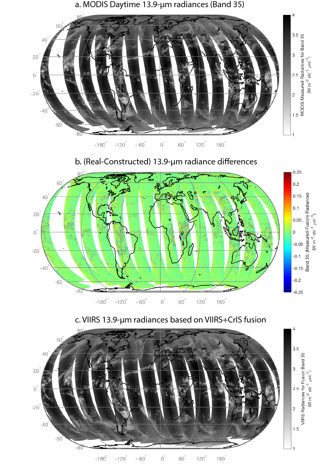
Figure 5: (a) Measured MODIS Band 35 (13.9-µm) daytime radiances for April 17, 2015. (b) MODIS Band 35 (measured – constructed) 13.9-µm radiance differences for the MODIS swath limited to sensor zenith angle ≤ 57˚. (c) Constructed 13.9-µm radiances for VIIRS based on CrIS data, for that portion of the VIIRS swath where there is complete CrIS coverage, i.e., sensor zenith angle ≤ 60˚.