[Section 2] [Home] [Section 4]
In this section we shall consider functions like z = f(x,y). These are represented by the MathType
The data for the quantities x and y will be given by a two-dimensional set. The first example is analog to our very first example (see sections 1.2 and 2.1), but with a two-dimensional domain. Our range might be interpreted as a surface (if range is composed of one RealType; range may of course be a RealTupleType) and it plays the role of the dependent variable. We shall, however start off with a 2D-display and shall map range to color.( (x, y) -> range )
where row and column, and pixel are RealTypes.( (row, column) -> pixel )
We organize (row, column) in a RealTupleType like the following
Our function, that is the pixel values for each row and column would bedomain_tuple = new RealTupleType(row, column)
func_dom_pix = new FunctionType( domain_tuple, pixel );
To define integer domain values (for the "domain_tuple") we use the class Integer2DSet:
This means, define the domain by constructing a 2-dimensional set with values {0, 1, ..., NROWS-1} x {0, 1, ..., NCOLS-1}. Note that these are integer values only.domain_set = new Integer2DSet(domain_tuple, NROWS, NCOLS );
We assume we have some NROWS x NCOLS pixel values in an array float[NROWS][NCOLS] (pixel values might be Java doubles, too). It is important to observe that the pixel samples are in raster order, with component values for the first dimension changing fastest than those for the second dimension. So, although the pixel values are in an array float[NROWS][NCOLS], they will be stored in a FlatField like float[1][NROWS * NCOLS]. One reason for doing this is computational efficiency.
Suppose we have an array with 6 rows and 5 columns, like
pixel_vals = {{0, 6, 12, 18, 24},
    	      {1, 7, 12, 19, 25},
	      {2, 8, 14, 20, 26},
	      {3, 9, 15, 21, 27},
	      {4, 10, 16, 22, 28},
	      {5, 11, 17, 23, 29}  };
then these values should be ordered as the values above indicate. This can be done by creating a "linear" array float[ 1 ][ number_of_samples ] (here called "flat_samples"), and then by putting the original values in this array. A way of doing this is can be seen in the following loops:
for(int c = 0; c < NCOLS; c++)

    for(int r = 0; r < NROWS; r++)

	     flat_samples[0][ c * NROWS + r ] = pixel_vals[r][c];
You can see how this is done in the code of example P3_01, as follows:
// Import needed classes

import visad.*;
import visad.java2d.DisplayImplJ2D;
import java.rmi.RemoteException;
import javax.swing.*;

/**
  VisAD Tutorial example 3_01
  A function pixel_value = f(row, column)
  with MathType ( (row, column) -> pixel ) is plotted
  The domain set is an Integer1DSet
  Run program with "java tutorial.s3.P3_01"
 */


public class P3_01{

// Declare variables
  // The quantities to be displayed in x- and y-axes: row and column
  // The quantity pixel will be mapped to RGB color

  private RealType row, column, pixel;

  // A Tuple, to pack row and column together, as the domain

  private RealTupleType domain_tuple;


  // The function ( (row, column) -> pixel )
  // That is, (domain_tuple -> pixel )

  private FunctionType func_dom_pix;


   // Our Data values for the domain are represented by the Set

  private Set domain_set;


  // The Data class FlatField

  private FlatField vals_ff;

  // The DataReference from data to display

  private DataReferenceImpl data_ref;

  // The 2D display, and its the maps

  private DisplayImpl display;
  private ScalarMap rowMap, colMap, pixMap;


  public P3_01(String []args)
    throws RemoteException, VisADException {

    // Create the quantities
    // Use RealType(String name);

    row = new RealType("ROW");
    column = new RealType("COLUMN");

    domain_tuple = new RealTupleType(row, column);

    pixel = new RealType("PIXEL");


   // Create a FunctionType (domain_tuple -> pixel )
   // Use FunctionType(MathType domain, MathType range)

    func_dom_pix = new FunctionType( domain_tuple, pixel);

    // Create the domain Set, with 5 columns and 6 rows, using an
    // Integer2DSet(MathType type, int lengthX, lengthY)

    int NCOLS = 5;
    int NROWS = 6;

    domain_set = new Integer2DSet(domain_tuple, NROWS, NCOLS );


    // Our pixel values, given as a float[6][5] array

    float[][] pixel_vals = new float[][]{{0, 6, 12, 18, 24},
    					 {1, 7, 12, 19, 25},
					 {2, 8, 14, 20, 26},
					 {3, 9, 15, 21, 27},
					 {4, 10, 16, 22, 28},
					 {5, 11, 17, 23, 29}  };

    // We create another array, with the same number of elements of
    // pixel_vals[][], but organized as float[1][ number_of_samples ]

    float[][] flat_samples = new float[1][NCOLS * NROWS];

    // ...and then we fill our 'flat' array with the original values

    // Note that the pixel values indicate the order in which these values
    // are stored in flat_samples

    for(int c = 0; c < NCOLS; c++)
      for(int r = 0; r < NROWS; r++)

	flat_samples[0][ c * NROWS + r ] = pixel_vals[r][c];


    // Create a FlatField
    // Use FlatField(FunctionType type, Set domain_set)

    vals_ff = new FlatField( func_dom_pix, domain_set);

     // ...and put the pixel values above into it

    vals_ff.setSamples( flat_samples );

    // Create Display and its maps

    // A 2D display

    display = new DisplayImplJ2D("display1");

    // Get display's graphics mode control and draw scales

    GraphicsModeControl dispGMC = (GraphicsModeControl) display.getGraphicsModeControl();
    dispGMC.setScaleEnable(true);


    // Create the ScalarMaps: column to XAxis, row to YAxis and pixel to RGB
    // Use ScalarMap(ScalarType scalar, DisplayRealType display_scalar)

    colMap = new ScalarMap( column, Display.XAxis );
    rowMap = new ScalarMap( row,    Display.YAxis );
    pixMap = new ScalarMap( pixel,  Display.RGB );

    // Add maps to display

    display.addMap( colMap );
    display.addMap( rowMap );
    display.addMap( pixMap );


    // Create a data reference and set the FlatField as our data

    data_ref = new DataReferenceImpl("data_ref");

    data_ref.setData( vals_ff );

    // Add reference to display

    display.addReference( data_ref );


    // Create application window and add display to window

    JFrame jframe = new JFrame("VisAD Tutorial example 3_01");
    jframe.getContentPane().add(display.getComponent());


    // Set window size and make it visible

    jframe.setSize(300, 300);
    jframe.setVisible(true);


  }


  public static void main(String[] args)
    throws RemoteException, VisADException
  {
    new P3_01(args);
  }

}
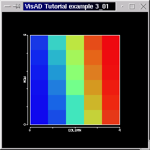
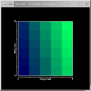
Running the program above (code available here) with "java tutorial.s3.P3_01" generates a window like the screen shot below.
Note again how the samples are organized. Remember that pixel values were mapped to RGB color. (Blue represents the smallest and red represents the largest.)
Our next example is almost like the previous example. We shall use, however, a Linear2DSet, which allows non-integer domain values, to define the 2-D domain set. First we rename the domain RealTypes "latitude" and "longitude", which are usually non-integer, since "row" and "column" suggest integer values (and an IntegerSet is indeed a sequence of consecutive integers).
In this example we shall consider the MathType
with the RealTypes latitude, longitude and temperature.( (latitude, longitude) -> temperature )
Our 2-D set will have the domain tuple:
domain_tuple = new RealTupleType(latitude, longitude);
Our set is
domain_set = new Linear2DSet(domain_tuple, 0.0, 6.0, NROWS,
                                           0.0, 5.0, NCOLS);
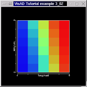
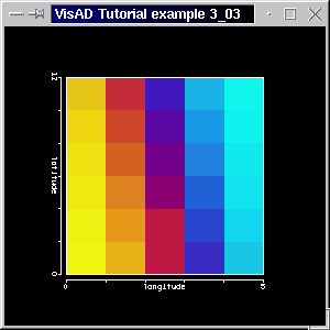
If you compile the program P3_02 and run it with "java tutorial.s3.P3_02" you should see the window below.
Before we change the DisplayRealType, we would like to draw attention to the parameters "first" and "last" of the previous example. We now define our set with
domain_set = new Linear2DSet(domain_tuple, 0.0, 12.0, NROWS,
                                           0.0,  5.0, NCOLS);
As we have said, we will not map to RGB, bur instead to Display.Red, simply by defining the ScalarMap
We also create two ConstantMapstempMap = new ScalarMap( temperature, Display.Red );
double green = 0.0;
double blue = 0.0;

greenCMap = new ConstantMap( green, Display.Green );
blueCMap  = new ConstantMap( blue, Display.Blue );
and add them to the display.
The reason for creating and adding these constant maps to the display is that the default values for green and blue is 1.0. (In fact, default values for red, green and blue are all 1.0, in order to create white graphics when color is not explicitely specified. See examples 1.1 and 2.3.)
The result of the above changes can be seen below. The code is available here.
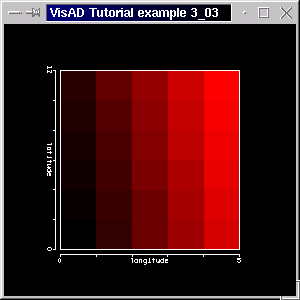
You could use Display.Cyan instead of Display.Red. This would result in a display with colors varying from red to black (rememeber, green and blue components are zero) like the display shown in the screenshot below:
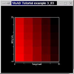
Note that the color varies from red to black. This is because in the RGB system cyan is defined as
cyan = white - redwhich can be rewritten in component form (red, green, blue):
(0,1,1) = (1,1,1) - (1,0,0)So when temperature is at the maximum (red = 1), cyan equals zero. Other subtractive color components are
magenta = white - greenand
yellow = white - blueYou can try these out, just uncomment the appropriate line in the code of example P3_03. For example, we create the map
with the constant mapstempMap = new ScalarMap( temperature, Display.Green );
This will set a constant level of blue across the entire display. See the screen shot below:double red = 0.0; double blue = 0.4; redCMap = new ConstantMap( green, Display.Red ); blueCMap = new ConstantMap( blue, Display.Blue );
Try decreasing the level of blue to 0.0 and see the change. (Remeber in the RGB system adding red and green gives yellow, adding red and blue gives magenta and adding blue and green gives cyan (blue-green).) Note that there's no red, but some blue.
One might use Display.Cyan instead of Display.Red. This would in a display with colors varying from red to black. (Actually, not quite totally black, because we have added a ConstantMap with some green.)
You should try out some other DisplayRealTypes. Just uncomment the appropriate lines in the code of example P3_03.
Using Display.CMY (Cyan, Magenta, Yellow) results in:
Using Display.Value (or Brightness) results in:
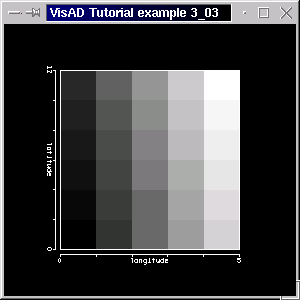
This would be similar to creating and adding the maps
without any other constant maps.tempRedMap = new ScalarMap( temperature, Display.Red ); tempGreenMap = new ScalarMap( temperature, Display.Green ); tempBlueMap = new ScalarMap( temperature, Display.Blue );
to( (latitude, longitude) -> temperature )
( (latitude, longitude) -> (temperature, pressure, precipitation) )
where the range (temperature, pressure, precipitation) is organized as a RealTupleType. We could use a constructor like
for our RealTupleType. When the range has many RealTypes you might want to use a handier constructor:RealTupleType( RealType temperature, RealType pressure, RealType precipitation);
That's how we create the RealTupleType for the range this example. We have the RealTypesRealTupleType( RealType[] my_realTypes);
temperature = new RealType("temperature");
pressure = new RealType("pressure");
precipitation = new RealType("precipitation");
RealType[] range = new RealType[]{ temperature, pressure, precipitation};

range_tuple = new RealTupleType( range );
Our function type is then
We use a Linear2DSet just like the one from the previous example (but with more samples and with different "first" and "last" values). We generate temperature, pressure and precipitation values in two for-loops and use some arbitrary functions (like sine, cosine, exponential). To set the sample values in the FlatFieldfunc_domain_range = new FunctionType( domain_tuple, range_tuple);
we need a "flat_samples" array of floats (although it might also be an array of doubles) just as float[ number_of_domain_components ][ number_of_range_components ], which is, in our casevals_ff = new FlatField( func_domain_range, domain_set);
This time we call FlatField.setSamples() with an extra parameterflat_samples = new float[3][NCOLS * NROWS];
vals_ff.setSamples( flat_samples , false );
As promised, we map temperature to red, pressure to green and precipitation to blue, as indicated by the following lines:
You can see the complete code here.tempMap = new ScalarMap( temperature, Display.Red ); pressMap = new ScalarMap( pressure, Display.Green ); precipMap = new ScalarMap( precipitation, Display.Blue );
Running the program will generate a window like the screen shot below:
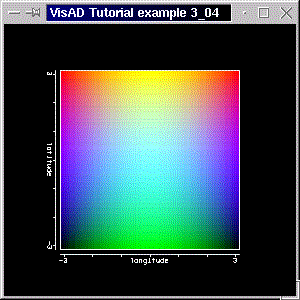
Note that temperature (red) has a maximum at the top and a minimum at the bottom of the display. Pressure (green) has a maximum along longitude=0, and precipitation along latitude=0, both decreasing exponentially as one moves away from their maximum. Also note how the red, green and blue values are added, creating different colors. It is important to realize the difference between mapping a quantity to Display.RGB and mapping to Display.Red, Display.Green and Display.Blue. The former makes use of a user-definable color table and the latter maps the quantitiy to both red, green and blue, scaling these components between 0 (quantity's minimum) to 1.0 (quantity's minimum) and adding them.
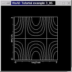
We will use a bigger Linear2DSet and will generate some values in the code. This is nothing really new. The (nice and) new feature of this example is the use of a new DisplayRealType:( (latitude, longitude) -> temperature )
You might have already guessed: this ScalarMap will calculate the isocontours of the associated RealType (in this case, temperature). The result is a display with white isolines (the isotherms). The IsoContour ScalarMap is added to the display, as usual. You can see the complete code here.tempIsoMap = new ScalarMap( temperature, Display.IsoContour );
Running the program will generate a window like the screen shot below:
If you want to colour the isolines according to the temperature, you simpy create and add the following map
In the code of example P3_05 the ScalarMap above has been created but not added to the display. Uncomment the linetempRGBMap = new ScalarMap( temperature, Display.RGB );
to add a RGB map, which will color the isolines like in the figure below:display.addMap( tempRGBMap );
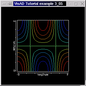
Note that the isolines are now colored according to temperature.
Note that we get the ContourControl from an IsoContour ScalarMap.ContourControl isoControl = (ContourControl) tempIsoMap.getControl();
    float interval = 0.1250f;  // interval between lines
    float lowValue = -0.50f;   // lowest value
    float highValue = 1.0f;    // highest value
    float base = -1.0f;        //  starting at this base value
While we still in control of the contours, we draw the contour labels too:isoControl.setContourInterval(interval, lowValue, highValue, base);
The result can be seen in the screen shot below. The code is available here.isoControl.enableLabels(true);
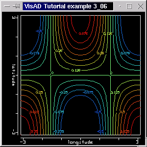
Note that we have denser isolines (due to the "interval"), which are drawn from -0.5 (lowValue) to 1.0 (highValue). Also note that the base lies below the lowValue. (It's possible to draw dashed lines below the base.) In the figure you can also see the labels showing the value at some isolines.
Although the ContourControl provides the control for how isolines should be depicted,
you might not want to have to set those parameters in your code. To avoid that,
VisAD also provides a user interface, the ContourWidget (please
see section 4.2), which is the interface
for the controls mentioned above and for a few more.
Before we carry on to combine a flat surface with the respective iso-contours a few comments.
You can also use the ContourControl to fill-in between the contours.
This is achieved by calling
This requires the RealType that is mapped to Display.IsoContour to be also mapped to Display.RGB, otherwise it won't work properly. I the next section, however, we draw contours on top of the surface by other means.isoControl.setContourFill(true);
We start with our previous example and add the new RealType, FunctionType, FlatField and DataReference
The RealType isoTemperature is defined asRealType isoTemperature; FunctionType func_domain_isoTemp; FlatField isoVals_ff; DataReferenceImpl iso_data_ref;
isoTemperature = new RealType("isoTemperature", SI.kelvin, null);
where the domain tuple is the RealTupleType formed by latitude and longitude.func_domain_isoTemp = new FunctionType( domain_tuple, isoTemperature);
we use the method FlatField.getFloats(boolean copy) to get the (float) temperature values (using copy = false in order not to copy the values).iso_vals_ff = new FlatField( func_domain_isoTemp, domain_set);
We then set the isocontours FlatField's samples withfloat[][] flat_isoVals = vals_ff.getFloats(false);
Again using an argument copy = false, to avoid copying the array. (Please note the we have created a "temporary" array float[][] flat_isoVals, but just for clarity's sake. We could have callediso_vals_ff.setSamples( flat_isoVals , false );
which does the same, but which is not very adequate for showing what is returned with the call FlatField.getFloats(boolean copy).)iso_vals_ff.setSamples( vals_ff.getFloats(false) , false );
The next steps are the creation of the ScalarMaps
and their addition to the display, as usual. We also create a DataReference, set its data and add to the displaytempIsoMap = new ScalarMap( isoTemperature, Display.IsoContour ); tempRGBMap = new ScalarMap( temperature, Display.RGB );
iso_data_ref = new DataReferenceImpl("iso_data_ref");
iso_data_ref.setData( iso_vals_ff );
display.addReference( iso_data_ref );
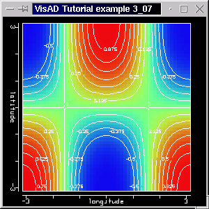
Note that the contours are drawn in white and they have the same interval, minimum and maximum value of the previous example. If you want contour lines of a quantity, e.g. temperature, drawn over the colored field of another quantity, e.g. pressure, than you'd only need to set pressure's FlatFields with pressure values (rather than copy the values, as we've done).
We have also drawn contour labels. Remeber, using an array of ConstantMaps you can set the isolines colors, as shown in section 2.4. We shall do that in the next example.
To create GMCWidget we simply do
where dispGMC is simply the GraphicsModeControl that was already available. We have chosen to add the GMCWidget to the same JFrame of the display (you may, of course, create a new JFrame for it).gmcWidget = new GMCWidget( dispGMC );
As promised, we color the contours we a constant (and dull) gray (75% of each red, green and blue component), by the means of an array of ConstantMaps:
ConstantMap[] isolinesCMap = { new ConstantMap( 0.75f, Display.Red ),
                               new ConstantMap( 0.75f, Display.Green ),
                               new ConstantMap( 0.75f, Display.Blue ) };
display.addReference( iso_data_ref, isolinesCMap );
The complete code for example P3_08 is available here. Running the program with "java tutorial.s3.P3_08" will generate a window like the screen shot below.
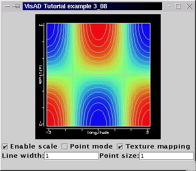
As you can see in the screen shot, the GMCWidget allows you to change line width and point size as well as select whether you want scales to be drawn, whether data should be rendered as points and whether you would like texture mapping. You should run example program P3_08 and try it out!
Note that we could have created a ScalarMap like
and have it added it to display to color the isolines. The necessary line are all available in the code for you to try out (although you won't see much of the isolines, as they have exactly the same color as the background; try changing their width and/or changing the colored field to point mode). don't forget to callisoTempRGBMap = new ScalarMap( isoTemperature, Display.RGB );
instead of calling it with the ConstantMaps.display.addReference( iso_data_ref, null );
which is almost like the previous one, only that the range (altitude, temperature) has now two RealTypes. We shall map the first RealType to IsoContour and the other to RGB. The result should be a display with the isolines (altitude contours), colored according to the temperature.( (latitude, longitude) -> (altitude, temperature) )
and the isolines are going to be colored according to the temperature because of the ScalarMapaltIsoMap = new ScalarMap( altitude, Display.IsoContour );
The two ScalarMaps are then added to the display, as usual. You can see the complete code here.tempRGBMap = new ScalarMap( temperature, Display.RGB );
Running the program will generate a window like the screen shot below:
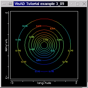
Note that the altitude isolines are colored according to temperature. (The altitude curve has a peak around the point (longitude, latitude) = (0, 0), otherwise the curve tends to zero. The color pattern is just like that of the screenshot in section 3.6.)
If you want to draw the isolines over the surface, then you have to split the MathType into two:
and( (latitude, longitude) -> altitude )
This is just what we did in section 2.7. We need two FunctionTypes as well as two FlatFields (and two float[1][ NCOLS * NROWS] samples arrays) and two DataReferences, one for altitude and the other for temperature.( (latitude, longitude) -> temperature )
Although the screen shot above is unusual in the sense that one does
not often color contours according to a quantity other than the contour
quantity itself (because it's a difficult thing to implement?), in VisAD
you're not bound to such "traditions". You are free to try out different
data depictions, and for that it generally suffices to change the
ScalarMaps (although not every choice of
DisplayRealType is legal). We do encourage you to try changing
the ScalarMaps and DisplayRealTypes (if you haven't
done it so far!) and for that we have provided some extra lines of code,
which you only have to uncomment, compile and run.
Looking at the screen shot again you might think it'd be better to
map temperature to color and altitude to the z-axis. Indeed it is! So by
now you should be asking yourself how you actually create a 3-D
display and how you map some RealType to the z-axis. This is
now a trivial issue: just create a 3-D display (rather than a 2-D one)
and map your RealType to Display.ZAxis. We'll do that
in the next section.